Quantum Basics¶

Hilbert space : $\mathcal H = \mathbb C^{2^n}$

wave function : $\ket \phi\in \mathcal H$

a spin-$\frac{1}{2}$ system, $\mathcal H=\mathbb C^2$, $\phi = \alpha\ket\uparrow+\beta \ket \downarrow\quad |\alpha|^2+|\beta|^2=1$
basic state : $\ket\uparrow =\begin{bmatrix}1\\0\end{bmatrix}\quad \ket \downarrow =\begin{bmatrix}0\\1\end{bmatrix}\quad \ket \rightarrow=\frac{1}{\sqrt 2}\begin{bmatrix}1\\1\end{bmatrix}$

pauli matrices : $\sigma_x=\begin{bmatrix}0&1\\1&0\end{bmatrix}~\sigma_y=\begin{bmatrix}0&-i\\i&0\end{bmatrix}~\sigma_z = \begin{bmatrix}1&0\\0&-1\end{bmatrix}$

$\sigma_i = \sigma_i^\dagger$ : Hermitian
$\sigma_i = \sigma_i^{-1}$ : involutory
$\sigma_i^2 = I$
$|\sigma_i|=-1$ : determinant
$\text{Tr}(\sigma_i) = 0$ : trace
$\lambda = \pm1$ : eigen values, eigen vectors are positive negative axes in Bloch sphere
$[\sigma_i,\sigma_j]=2i\epsilon_{ijk}\sigma_k$ : commutation, $\epsilon_{ijk}$ : Levi-Civita symbol
$\{\sigma_i,\sigma_j\} = 2\delta_{ij}I$ : anti-commutation, $\delta_{ij}$ : kronecker delta

Operators :

spin operator : $\hat S_x = \frac{\hbar}{2}\sigma_x\quad\hat S_y=\frac{\hbar}{2}\sigma_y\quad \hat S_z=\frac{\hbar}{2}\sigma_z$
spin pointing along direction $\vec e =\begin{bmatrix}e_x,e_y,e_z\end{bmatrix}$ $\vec e\cdot\hat {\vec S}=\frac{\hbar}{2}\begin{bmatrix}e_z&e_x-ie_y\\e_x+ie_y&-e_z\end{bmatrix}$
position operator : $\hat q\ket {\psi(q)} = q\psi(q)$
momentum operator : $\hat p = -i\hbar \frac{\text d}{\text d q}$
hamiltonian operator : $\hat H = -\frac{\hbar^2}{2m}\nabla^2 + V$
kinetic operator : $\hat T = \frac{\hat{(\vec p)}^2}{2m} = \frac{-i\hbar ^2}{2m}\nabla^2$
potential operator : $\hat V = V$

Schrödinger equation ：$i\hbar \partial_t \ket{\psi(t)}=\hat H\ket {\psi(t)}$

for stationary problem : $\hat H \ket \psi = E\ket\psi\quad \psi(t)=e^{-iEt/\hbar}\ket {\psi(0)}$
external potential : $i\hbar\partial_t\psi(\hat r)=-\frac{\hbar^2}{2m}\nabla^2\psi(\vec r)+V(\vec r)\psi(\vec r)$

Notation

$\hat H$ Hamilton operator

$E$ energy of the system

$V$ potential

Example

harmonic oscillator : $\frac{1}{2}(\hat p^2+\hat q^2)\ket \psi = E \ket \psi$

$V(\hat q) = \frac{1}{2}\hat q^2$

$\psi(q)=\frac{1}{\sqrt{2^nn!\sqrt{\hbar\pi}}}e^{-q^2/2}H_n\left(\frac{1}{\sqrt \hbar}q\right)$

$E = \hbar (n+\frac{1}{2})$

Density matrix : $\hat \rho = \sum_{i,j}p_{i,j}\ket{\psi_i}\bra{\psi_j}$

purity of the system $\text{Tr}(\hat \rho^2)$
for a pure state without noise : $\hat \rho_{\text{pure}}=\ket\psi\bra\psi$

Example

$\hat\rho_{\rightarrow} = \ket{\rightarrow}\bra{\rightarrow}=\begin{bmatrix}\frac{1}{2}&\frac{1}{2}\\\frac{1}{2}&\frac{1}{2}\end{bmatrix}$

$\text{Tr}(\hat \rho_\rightarrow)=1$

$\hat \rho_{\uparrow\downarrow}= \ket{\uparrow}\bra{\downarrow}=\begin{bmatrix}\frac{1}{2}&0\\0&\frac{1}{2}\end{bmatrix}$

$\text{Tr}(\hat \rho_{\uparrow\downarrow})=\frac{1}{2}$

unitary time evolution : $i\hbar \partial_t\hat\rho(t)=[\hat H,\hat\rho(t)]$
thermal density matrix : $\hat \rho_\beta = \frac{1}{\sum_i e^{-\beta E_i}}\sum_i e^{-\beta E_i}\ket i\bra i = \frac{1}{\text{Tr}(e^{-\beta \hat H})}e^{-\beta \hat H}$

measurement : $\bra \psi \hat A \ket \psi = \text{Tr}(\hat \rho \hat A)$

measure non commute operator : $[\hat A,\hat B]=i\hbar\Leftrightarrow \Delta A\cdot \Delta B \ge \frac{\hbar}{2}$

Quantum 1-body problem¶

given $V$ ,we want to know $\psi$ according to Schrödinger equation $-\frac{\hbar^2}{2m}\partial_x^2\psi(x)+V(x)\psi(x)=E\psi(x)$

Time-Independent 1 D Schrödinger equation¶

stationary assumption : $\psi(t)=e^{-iEt/\hbar}\ket {\psi(0)}$ $$ -\frac{\hbar^2}{2m}\nabla2\psi(x) + V(x)\psi(x) = E\psi(x) \to H\psi(x) = E\psi(x) $$

for special form $$ \psi''(x) + \frac{2m}{\hbar^2}\left(E-V(x)\right)\psi(x) = 0 $$

given $V,m,E$ we want to know $\psi$

Numerov algorithm $$ \begin{aligned} \left(1+\frac{(\Delta x)^2}{12}k_{n+1}\right)\psi_{n+1} &= 2\left(1-\frac{5(\Delta x)^2}{12}k_n\right)\psi_n - \left(1+\frac{(\Delta x)^2}{12}k_{n-1}\right)\psi_{n-1} + O[(\Delta x)^6] \ k &= \frac{2m}{\hbar^2}(E-V(x)) \end{aligned} $$

initial problem for symmetry $V(x)=V(-x)$
$\psi(x)=-\psi(x)$ : half integer mesh with $\psi(-\frac{1}{2}\Delta x) = \psi(\frac{1}{2}\Delta x) = 1$
$\psi(-x) = -\psi(x)$ : integer mesh with $\psi(0) = 0 \quad \psi(\Delta x) = 1$
general $V(x)=0$ for $|x|\ge a$
$\psi(-a-\Delta x) = \text{exp}(-\Delta x\sqrt {-2mE}/\hbar)\quad \psi(-a)=1$

1D scattering problem

a particle approaching the potential barrier $V(x)\begin{cases} \neq 0 & x\in[0,a]\\ = 0 & \text{others} \end{cases}$ from the left

1D scattering potential

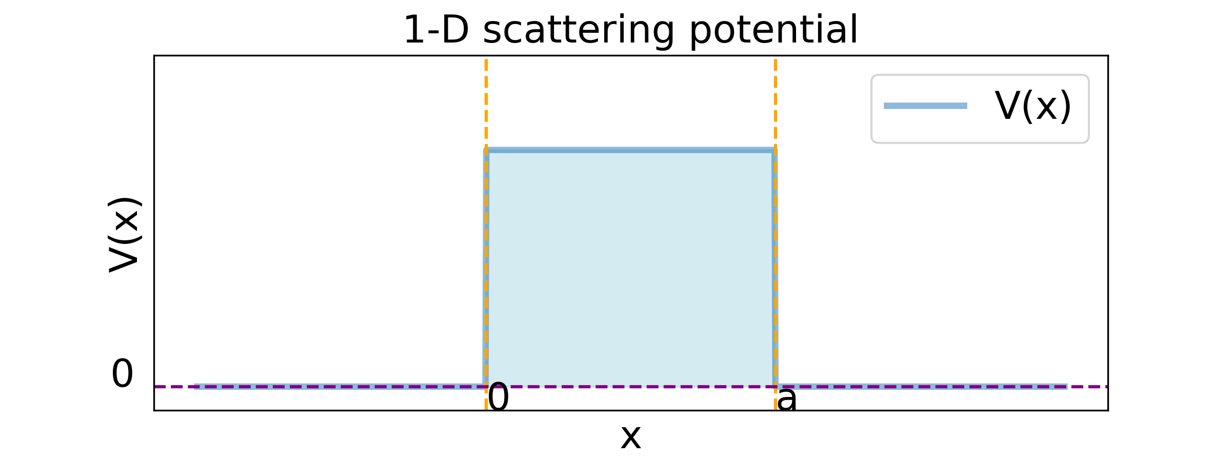
wave function assumptions :
left ($x<0$) wave function : $\psi_L(x) = \underbrace{Ae^{iqx}}_{\text{origin wave}}+\underbrace{Be^{-iqx}}_{\text{reflection}}$
right ($x>a$) wave function : $\psi_R(x) = \underbrace{Ce^{iqx}}_{\text{transmission}}$
where $q$ is the wave number $q^2 = \frac{2m[E-V(x)]}{\hbar^2}$
solution :

Algorithm

set $C=1$, use Numerov algorithm starting at $a+\Delta x$ from right to left

match the numerical solution on the left $x<0$ to determine $A$ and $B$

probability :
reflection probaility : $R = \frac{|B|^2}{|A|^2}$
transition probability : $T = \frac{|C|^2}{|A|^2}$

Bound state

particles are confined due to potential $V(x)\begin{cases}<0&x\in[0,a]\\= 0&\text{others}\end{cases}$

1D bound state potential

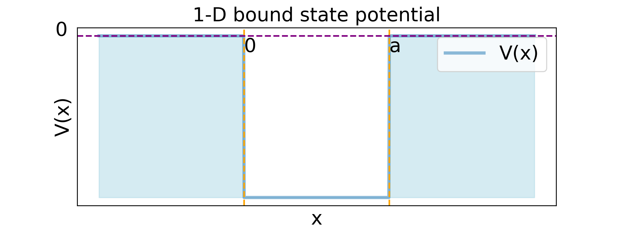
shooting method for eigen solver

Algorithm

try a energy $E$

use numerov algorithm from $x=0$ to $x_f\gg a$

satisfy $\psi_E(x_f)\approx 0$ then $E$ is a eigenvalue else try another $E$

Improved Method - Integration from Both Sides

Algorithm

try a position $b\in (0,a)$ , that $E=V(b)$, $\frac{\partial^2 \psi_E}{\partial x^2} = 0$

use numerov from $a$ to $b$ as $\psi_L$ and from $0$ to $b$ as $\psi_R$

satisfy $\frac{\psi'_L(b)}{\psi_L(b)}=\frac{\psi'_R(b)}{\psi_R(b)}$ ($\psi_L,\psi_R$ are not normalized ), then $E$ is a eigenvalue else try another $b$

Time-independent nD Schrödinger equation¶

Factorization techniques :

along coordinate axes : $\psi(\vec r) =\psi_x(x)\psi_y(y)\psi_z(z)$
spherical symmetry : $\psi(\vec r) = \frac{u(r)}{r}Y_{lm}(\theta,\phi)\quad l\in\N_0,m\in\Z,|m|\le l$

apply to the Schrodinger equation : $\left(-\frac{\hbar^2}{2\mu}\nabla^2+\frac{\hbar^2l(l+1)}{2\mu r^2}+V(r)\right)u(r) = Eu(r)$

Notation

$l$ : azimuthal quantum number, magnitude of the orbital angular momentum

$m$ : magnetic quantum number, projection of the angular momentum vector along a chosen axis

$\mu$ : mass

Solving methods :

finite difference

Example : three dimensional Schrodinger $$ \nabla^2\psi(\vec r) + 2m[E-V(\vec r)]\psi(\vec r) = 0 \ \Downarrow \ \begin{aligned} 0 = \frac{1}{(\Delta x)^2}&[\psi(x_{n+1},y_n,z_n)+\psi(x_{n-1},y_n,z_n)\ &+\psi(x_n,y_{n+1},z_n)+\psi(x_n,y_{n-1},z_n)\ &+\psi(x_n,y_n,z_{n+1})+\psi(x_n,y_n,z_{n-1}) ]\ &+\left{ 2m[E-V(\vec r)]-\frac{6}{(\Delta x)^2} \right}\psi(x_n,y_n,z_n) \end{aligned} $$

variational approaches : $\ket \phi = \sum_i^N a_i\ket {u_i}$ $$ \braket{\phi}E^* = \bra \phi \hat H \ket \phi \to \underbrace{\bra{u_i}\ket{u_j}}{S}} E^* = \underbrace{\bra{u_i}\hat H\ket{u_j}{H \to U^\top HU\hat b = E^*\vec b $$}

more basis more accurate

Notation

$\ket{u_i}$ basis

$a_i$ : basis coefficient, $\vec a = \begin{bmatrix}a_1,\cdots,a_n\end{bmatrix}^\top$

$U$ : nomalization matrix for $S$ that $U^\top SU = I$

$\vec b$ : eigen vector, $\vec b = U^{-1}\vec a$

finite element method
irregular geometries
higher accuracy

Time dependent Schrödinger Equation¶

\[ i \partial_t \ket \psi = \hat H\ket \psi \]

Spectral method ：$\ket{\psi_t} = \sum_n c_ne^{-i\varepsilon_n(t-t_0)/\hbar}\ket {\phi_n}$

Algorithm

eigen value $\varepsilon_n$ and eigen vector $\ket {\phi_n}$ for stationary problem $\hat H\ket \phi = E\ket \phi$

represent initial wave function in eigen vectors $\ket {\psi_0} = \sum_n c_n \ket{\phi_n}$

the evolution state $\ket{\psi_t} = \sum_n c_ne^{-i\varepsilon_n(t-t_0)/\hbar}\ket {\phi_n}$

limitations :

the diagonalization of $H$ is complex, so this method is only useful for small problems

Notation

$\ket {\phi_n}$ : eigenvector of $H |ϕ⟩ = E |ϕ⟩$, $\ket {\psi_0} = \sum c_n\ket{\phi_n}$

$\varepsilon_n$ : eigenvalue of $H |ϕ⟩ = E |ϕ⟩$

Direct numerical integration : $\left(\mathbb 1+ \frac{i\Delta t}{2\hbar}H\right)\psi(\vec r, t+\Delta t) = \left(\mathbb 1 - \frac{i\Delta t}{2\hbar}H\right)\psi(\vec r, t)$

forward euler : $\ket {\psi(t_{n+1})}=\ket {\psi(t_n)} - \frac{i\Delta t}{\hbar}\hat H\ket{\psi(t_n)}$
numerically unstable
violet conservation of $\braket \phi$
implicit method : $\left(\mathbb 1+ \frac{i\Delta t}{2\hbar}H\right)\psi(\vec r, t+\Delta t) = \left(\mathbb 1 - \frac{i\Delta t}{2\hbar}H\right)\psi(\vec r, t)$
$H$ is sparse matrix, using iterative solver (e.g. biconjugate gradient)

Split-operator method : $\psi(\vec q) \xrightleftharpoons[\mathcal F^{-1}]{\mathcal F}\psi(\vec p)\Rightarrow \hat H =\textcolor{cyan}{\hat T(\vec p)}+\textcolor{magenta}{\hat V(\vec q)}$ $$ e^{-i t\hat H /\hbar} = \textcolor{magenta}{e^{-i\Delta t\hat V/2\hbar}}\left[\textcolor{cyan}{e^{-i\Delta t\hat T/\hbar}}\textcolor{magenta}{e^{-i\Delta t\hat V/\hbar}} \right]^{{N-1}\textcolor{cyan}{e} $$}}\textcolor{magenta}{e^{-i\Delta t\hat V/2\hbar}

Algorithm

$\textcolor{magenta}{\psi(\vec q)\gets e^{-i\Delta tV(\vec q)/2\hbar}\psi_0(\vec q)}$

loop N-1 timesteps

$\textcolor{cyan}{\psi(\vec p)} \overset{ \mathcal F}{\gets} \textcolor{magenta}{\psi(\vec q)}$

$\textcolor{cyan}{\psi(\vec p) \gets e^{-i\Delta t \hbar\Vert\vec p\Vert^2/2m}\psi(\vec p)}$

$\textcolor{magenta}{\psi(\vec q)} \overset{\mathcal F^{-1}}\gets \textcolor{cyan}{\psi(\vec p)}$

$\textcolor{magenta}{\psi(\vec q)\gets e^{-i\Delta t V(\vec q)/\hbar}\psi(\vec q)}$

$\textcolor{cyan}{\psi(\vec p)} \overset{\mathcal F}{\gets}\textcolor{magenta}{\psi(\vec q)}$

$\textcolor{cyan}{\psi(\vec p) \gets e^{-i\Delta t \hbar\Vert\vec p\Vert^2/2m}\psi(\vec p)}$

$\textcolor{magenta}{\psi(\vec q)} \overset{\mathcal F^{-1}}{\gets} \textcolor{cyan}{\psi(\vec p)}$

$\textcolor{magenta}{\psi(\vec q)\gets e^{-i\Delta t V(\vec q)/2\hbar}}$

Notation

$\vec p$ : momentum in hamilton expression

$\vec q$ : position in hamilton expression

$\hat T$ : kinetic operator , $\hat T = \frac{\hat{(\vec p)}^2}{2m} = \frac{-i\hbar ^2}{2m}\nabla^2$

$\hat V$ : potential operator , $\hat V = V$

$\mathcal F$ : fourier operator , $\mathcal F \psi(\vec q) = \left(\frac{1}{\sqrt {2\pi}}\right)^d\int_{-\infin}^{+\infin}\psi(\vec q)e^{-i\vec p\cdot \vec q}\text d\vec q$

$\mathcal F^{-1}$ : inverse fourier operator , $\mathcal F^{-1} \psi(\vec p) = \left(\frac{1}{\sqrt {2\pi}}\right)^d\int_{-\infin}^{+\infin}\psi(\vec p)e^{-i\vec p\cdot \vec q}\text d\vec p$

Quantum n-body problem¶

Hilbert space for n particles: $\mathcal H^N = \mathcal H^{\otimes N}$

Indistinguishable Particles¶

Bosons and Fermions :

fermions : $\psi(\vec r_1,\vec r_2) = -\psi(\vec r_2, \vec r_1)$

\[ \Psi^A = \mathcal N_A\sum_p\text{sign}(p)\psi(\vec r_{p(1)},\cdots,\vec r_{p(N)}) \]
Notation
- $\Psi^A$ : n particle fermions wave function
- $\mathcal N_A$ : normalization factor
- $p$ : permutation
- Pauli exclusion principle : $\Psi^A(\vec r_1,\vec r_2) = \psi(\vec r_1,\vec r_2)-\psi(\vec r_2,\vec r_1) \neq 0$
- spinful, generalized coordinate $r=(\vec r, \sigma)$
bosons : $\psi(\vec r_1, \vec r_2) = \psi(\vec r_2, \vec r_1)$

\[ \Psi^{S} = \mathcal N_S\sum_p \psi(\vec r_{p(1)},\cdots,\vec r_{p(N)}) \]
Notation
- $\Psi^S$ : n particle bosons wave function
- $\mathcal N_S$ : normalization factor

Fock space: $\mathcal F = \bigoplus_{N=0}^\infin \mathcal S_{\pm}\mathcal H^N$

possible particle configurations for a given type of particle

$\mathcal F = \underbrace{\mathcal F_0}_{\text{0 particles}} \oplus \underbrace{\mathcal F_1}_{\text{1 particles}} \oplus \cdots$

Notation

$\oplus$ : direct sum, e.g. $\textbf A \oplus \textbf B = \begin{bmatrix}\textbf A&\textbf 0\\\textbf 0 &\textbf B\end{bmatrix}$

$S_\pm$ : symmetrization for bosons $\mathcal S_+ =\mathcal N_S\sum_p$ / antisymmetrization operator for fermions $\mathcal S_- = \mathcal N_A\sum_p\text{sgn(p)}$

Example

Bosons Spinless Fermions Spinful Fermions Spin-$\frac{1}{2}$

Fock space dimension $\infin$(bosons can take same position) $2^N$ $4^N$ $2^N$

Slater determinant :$ \Psi(r_1,\cdots,r_N) = \frac{1}{\sqrt {N!}}\left|\begin{matrix} \phi_1(r_1)&\cdots&\phi_N(r_1)\ \vdots & \ddots&\vdots\ \phi_r(r_N)&\cdots&\phi_N(r_N) \end{matrix}\right| $

anti-symmetrized and normalized $N$ single particle wave function product

Notation

$\phi_i(r_j)$ : wave function of fermion $i$ at position $r_j$

Creation and annihilation operators

$\hat a$ annihilation operator : remove particle $\hat a_i\ket {\phi_j} = \delta_{ij}\ket {0}$
$\hat a^\dagger$ creation operator : add particle $\ket{\phi_i} = \hat a_i^\dagger \ket {0}$

Notation

$\ket {0}$ : vacuum state with no particles, $\ket {0} = \begin{bmatrix}0\\0\end{bmatrix}$

$[\cdot,\cdot]$ : commute, $[A,B]=AB-BA$

$\{\cdot,\cdot\}$ : anti-commute, $\{A,B\}=AB+BA$

Bosons : commute
$\hat a_i\ket{n_i}=\sqrt{n_i}\ket{n_i-1} \quad \hat a_i^\dagger \ket {n_i} = \sqrt {n_i+1}\ket{n_i+1}$
$\hat a_i^\dagger\hat a_i = n_i$
$[\hat a_i, \hat a_j^\dagger] = \delta _{ij}\quad [\hat a_i, \hat a_j] = [\hat a_i^\dagger, \hat a_j^\dagger] = 0$
$0\underset{\hat a}{\not\leftarrow}\ket 0 \xrightleftharpoons[\hat a]{\hat a^\dagger}\ket 1\xrightleftharpoons[\hat a]{\hat a^\dagger}\ket 2\cdots$
Fermions : anti-commute
$\hat c_{u_i}\ket{u_i,u_j,\cdots}=\ket{u_j,\cdots} \quad \hat c_{u_i}\ket{u_j,\cdots} = \ket{u_i,u_j,\cdots}$
$\hat c_i^\dagger\hat c_i =\hat n_i$
- $n_i = 0$ : $\hat c_i^\dagger\hat c_i\ket{u_j,\cdots} = 0$
- $n_i=1$ : $\hat c_{u_i}^\dagger\hat c_{u_i}\ket{u_i,u_j,\cdots}=\ket{u_i,u_j,\cdots}$
$\{\hat c_i, \hat c_j^\dagger\} = \delta_{ij}\quad \{\hat c_i, \hat c_j\} = \{\hat c_i^\dagger, \hat c_j^\dagger\} = 0$
$0 \underset{\hat c^\dagger_{u_i}}{\not \leftarrow}\ket 0 \xrightleftharpoons[\hat c_{u_i}]{\hat c^\dagger_{u_i}}\ket {u_i}\overset{\hat c^\dagger_{u_i}}{\not\rightarrow} 0$

Quantum Spin Model¶

(TFIM)Transverse field Ising model $$ \hat H = \sum_{} J_{ij} \hat S_i^z\hat S_j^z - \sum_{i} \frac{h_i}{2}\hat S_i^x $$

\[ \hat S_i^z\hat S_{j}^z = I\otimes\cdots \otimes \underbrace{\hat S^z}_{n=i}\otimes\cdots\otimes \underbrace{\hat S^z}_{n=j}\otimes\cdots\otimes \mathbb 1I \]

quantum phase transition between a spontaneously symmetry-broken and a disordered phase
extension of the classical Ising model by adding a magnetic field in the $x$ direction

Notation

$<ij>$ : connection between particle $i$ and particle $j$

$J_{ij}$ : interacting constant between particle $i$ and particle $j$

$h_i$ : external magenatic field on particle $i$

$\hat S^x$ : spin operator in $x$ direction, $\hat S^x = \frac{1}{2}\hbar\sigma_x = \frac{1}{2}\hbar\begin{bmatrix}0&1\\1&0\end{bmatrix}$

$\hat S^z$ : spin operator in $z$ direction, $\hat S^z = \frac{1}{2}\hbar \sigma_z = \frac{1}{2}\hbar\begin{bmatrix}1&0\\0&-1\end{bmatrix}$

Heisenberg model $$ \begin{aligned} \hat H &= \sum_{} J_{ij}\hat{\vec S_i}\cdot \hat{\vec S_j} = \sum_{}J_{ij}\left(\hat S^x_i \hat S^x_j +\hat S^y_i\hat S^y_j+\hat S^z_i\hat S_z^j\right) \ &= \sum_{}J_{ij}\left[ \frac{1}{2} \left(\hat S_i^+\hat S_j^- + \hat S_i^- \hat S_j^+\right) + \hat S_i^z \hat S_j^z \right] \end{aligned} $$

Notation

$\hat S^\pm$ : raising/lowering operator , $\hat S^\pm = \hbar \sigma^\pm =\hbar(\sigma_x\pm i \sigma_y)$

$\hat S^+ \hat S^+ \ket \downarrow = \hat S^+\ket \uparrow = \ket {\text{null}} \quad \ket{\uparrow} = \begin{bmatrix}1\\0\end{bmatrix}\qquad \ket{\downarrow} = \begin{bmatrix}0\\1\end{bmatrix}\qquad\ket{\text{null}} = \begin{bmatrix}0\\0\end{bmatrix}$

$(\sigma^\pm)^2= 0$ : a spin can be flipped only only once

$\hat M^z$ : total magnetization , $\hat M^z=\sum_i \hat S_i^z$

conserve total magentization
Hamitonian has $SU(2)$ symmetry

Example : two particles ($\{\ket{\uparrow\uparrow}, \ket{\uparrow\downarrow},\ket {\downarrow\uparrow}, \ket{\downarrow\downarrow}\}$)

$\hat H = \begin{bmatrix}\frac{1}{4}J_{ij}&0&0&0\\0&-\frac{1}{4}J_{ij}&\frac{1}{2}J_{ij}&0\\0&\frac{1}{2}J_{ij}&-\frac{1}{4}J_{ij}&0\\0&0&0&\frac{1}{4}J_{ij}\end{bmatrix}$

$XXZ$ model $$ \hat H = \sum_{}J_{ij}\left( \hat S_i^x\hat S_j^x + \hat S_i^y\hat S_j^y + \Delta\hat S_i^z\hat S_j^z \right) $$

conserve total magentization $\hat M^z$

Notation

$\Delta$ : hyperparameter

$\Delta = 0$ $\Delta = 1$ $\Delta\to \infin$

$XY$ model Heisenberg model Ising model

Jordan-Wigner Transformation

mapping spin models to spinless fermions, derive from $XXZ$ model $$ \hat H = \frac{1}{2}\sum_{}J_{ij}\left( \hat c_i^\dagger\hat c_j +\hat c_j^\dagger\hat c_i+ 2\Delta\hat n_i\hat n_j \right) $$

Notation

$\hat c_i/\hat c_i^\dagger$ : Jordan-Wigner transformation operator, $\hat c_i = \prod_{j<i}\left(\sigma_j^z\right)\sigma_i^+ \qquad \hat c_i^\dagger = \prod_{j<i}\left(\sigma_j^z\right)\sigma_i^-$

$\{\hat c_i,\hat c_j^\dagger\}=\delta_{ij}$

$\{\hat c_i, \hat c_j\}=\{\hat c_i^\dagger, \hat c_j^\dagger\}=0$

$\hat n_i$ : number operator, $\hat n_i=\hat c_i^\dagger \hat c_i$

Brute-force method¶

[ED] Exact Diagonalization¶

diagonalizing the Hamiltonian matrix

full spectrum $N\approx 20$
Lanczos algorithm $N\approx 40$

Lanczos algorithm

storage complexity $\mathcal O(2^N)$ compared to dense matrix eigen solvers of $\mathcal O(2^N)^2$
ghost state : low-lying eigen values result from round of error that $\vec r_n$ is not fully orthogonal

Algorithm

find the orthogonalized basis $\vec r_i$ using Gram-Schmidt orthogonalization

$\begin{aligned} \vec r_0 = \frac{\vec v}{\Vert \vec v\Vert} \quad \beta_m\vec r_m = H\vec r_{m-1} - \alpha_{m-1}\vec r_{m-1} - \beta_{m-1}\vec{r}{m-2} \end{aligned}\quad \alpha_n =\vec r_n^\dagger H\vec r_n \quad \beta_n = |\vec r_n^\dagger H\vec r| $

express Hamiltonian $H$ in tridiagonal matrix

$H^M = \begin{bmatrix} \alpha_0 & \beta_1 & \cdots & 0 & 0 \\ \beta_1 & \alpha_1 & \cdots & 0 & 0 \\ \vdots & \vdots & \ddots & \vdots & \vdots\\ 0 & 0 & \cdots & \alpha_{M-1}&\beta_M \\ 0 & 0 & \cdots & \beta_M & \alpha_M \end{bmatrix}$

eigendecomposite the $H^M$

transform the eigenvectors to the original basis

for memory constraint, only store the last three $\vec r_n$ and recompute $\vec r_n$ iteratively to perform basis transformation

Spin-$\frac{1}{2}$ hamitonians

two possible state $\ket\uparrow$ and $\ket\downarrow$ bitwise operation (xor) rather than vector

$\hat S_i^z\hat S_{i+1}^z$ : s = s ^ (s>>1)
$\hat S_i^+\hat S_{i+1}^-$ : s = s ^ (3<<i)

Example

assume state $s=011_2$

then for heisenberg model $\tilde s = 011 _2\oplus 010_2 = 010_2$ where $\oplus$ is bitwise xor here.

Notation

$\hat S^\pm$ : $\hat S^\pm = \hbar \sigma^\pm =\hbar(\sigma_x\pm i \sigma_y)$

symmetries

block diagonalize the Hamitonian and solve within the symmetries' eigenspaces.

Example : Transverse Field Ising Model

parity operator : $\hat P = \bigotimes_i \sigma_i^x$, the eigen values are $\pm 1$

$\ket \psi = \hat P^M \ket \psi$ : for random state $\psi$, apply operator for $M$ times we find the initial state again

eigen state becomes : $\sum_{i=0}^M\hat P^i\ket\psi$

construct hamiltonian $H$ from eigen state and eigen vector

Time evolution¶

Trotter-Suzuki decomposition: $\hat H = \sum_{k=1}^K \hat h_k\to e^{-i\hat H\Delta t/\hbar}= \prod_{k=1}^K e^{-i\hat h_k\Delta t/\hbar}+\mathcal O(\Delta t^2)$

time-indepedent assumption : $\ket{\psi(t+\Delta t)}= e^{-i\hat H\Delta t/\hbar}\ket{\psi(t)}$
non-commuting decomposition : $\hat H = \sum_{k=1}^K\hat h_k\quad [\hat h_i,\hat h_j]\neq 0\quad i\neq j$
second order version : $e^{-i\hat H\Delta t/\hbar} = \left(\prod_{k=1}^K e^{-i\hat h_k\Delta t/2\hbar}\right)\left(\prod_{k=K}^1 e^{-i\hat h_k\Delta t/2\hbar}\right)+\mathcal O(\Delta t^3)$

Example : $K=2$

$\ket{\psi(t+\Delta t)} = e^{-i\hat h_1 \Delta t/2\hbar}e^{-i\hat h_2\Delta t/\hbar}e^{-i\hat h_1\Delta t/2\hbar}\ket{\psi}$

Example : Transverse Field Ising Model

$\hat H = \underbrace{\sum_{<ij>}J_{ij}\sigma_i^z\sigma_j^z}_{\hat h_1} - \underbrace{\sum_i h_i\sigma_i^x}_{\hat h_2}$

$e^{-i\hat h_1\Delta t/\hbar} = \bigotimes_{<ij>}e^{-i\Delta tJ_{ij}s_i^z s_j6z/\hbar}$

$e^{-i\hat h_2\Delta t/\hbar} = \begin{bmatrix}\text{cos}(\Delta th_i/\hbar)&i\text{sin}(\Delta t h_i/\hbar)\\ i\text{sin}(\Delta th_i/\hbar)&\text{cos}(\Delta t h_i/\hbar)\end{bmatrix}$

(since $e^A = 1 + A + \frac{A^2}{2!}+\cdots$ )

Notation

$[\cdot,\cdot]$ : commute operator, $[A,B]=AB-BA=0\to A,B$ commute

$<i,j>$ : means $i,j$ are neighbors

$J_{ij}$ : connection between site $i$ and $j$

$h_i$ : magenatic field at site $i$

$\hat h_k$ : non-commuting term

$s_i$ : eigen value for $\sigma^z_i$

Imaginary-time evlotion: $it\to \tau$

time-indepedent assumption : $\ket{\psi(t)}= e^{-i\hat Ht/\hbar}\ket{\psi(0)}\to \ket{\psi(t)}=e^{-\tau\hat H}\ket{\psi(0)}$
converges to the ground state by suppressing the amplitudes of excited states exponentially fast in the product $\Delta E_k\tau$ .

Magnus expansian : $\hat U(\Delta t) = e^{-i\bar H_t\Delta t/\hbar}+\mathcal O(\Delta t^2)\quad H_t = \bar H_t^1 +\bar H_t^2+\cdots$

time-depdent assumption : $\ket{\psi(t')}=U(t',t)\ket{\psi(t)}$
$\bar H^1_t = \frac{1}{\Delta t}\int_{t}^{t+\Delta t} \hat H(s)ds$ and $H^2_t = -\frac{i}{\Delta t}\int_{t}^{t+\Delta t}ds\int_{t}^sdl\left[\hat H(s),\hat H(l)\right]$

Notation

$U$ : evolution operator, $\hat U(t',t) = e^{-i\int_t^{t'}\hat H(s)\text ds/\hbar}\quad t'>t$

Matrix Product States¶

Bipartite entanglement¶

Reduced density matrix : $\rho_A =\text{Tr}_B(\ket \psi \bra\psi)\quad \ket\psi \in\mathcal H =\mathcal H_A\otimes \mathcal H_B$

Notation

$\otimes$ : kronecker product, e.g. $\begin{bmatrix}1&0\\0&1\end{bmatrix}\otimes \begin{bmatrix}1&1\\1&1\end{bmatrix}=\begin{bmatrix}1&1&0&0\\1&1&0&0\\0&0&1&1\\0&0&1&1\end{bmatrix}$

$\text{Tr}_B$ : partial trace over subsystem $B$ , e.g. $\text{Tr}_B\begin{bmatrix}A_{11}B_{11}&A_{11}B_{12}&A_{12}B_{11}&A_{12}B_{12}\\A_{11}B_{21}&A_{11}B_{22}&A_{12}B_{21}&A_{12}B_{22}\\A_{21}B_{11}&A_{21}B_{12}&A_{22}B_{11}&A_{22}B_{12}\\A_{21}B_{21}&A_{21}B_{22}&A_{22}B_{21}&A_{22}B_{22}\end{bmatrix}=\begin{bmatrix}\sum_{ii}B_{ii}A_{11}&\sum_{ii}B_{ii}A_{12}\\\sum_{ii}B_{ii}A_{21}&\sum_{ii}B_{ii}A_{22}\end{bmatrix}$

Entanglement : $S=-\text{Tr}(\rho_A~ \text{log}~\rho_A)=-\text{Tr}(\rho_B~\text{log}~\rho_B)$

using Schmidt decomposition $\rho_A = \sum_\alpha \lambda_\alpha^2 \ket{\phi_\alpha}_A\bra{\phi_\alpha}_A\to S-\sum_\alpha \lambda_\alpha^2\text{log}\lambda_\alpha^2$

product state (zero entanglement) : $S=0\Leftrightarrow\lambda_1 = 1,\lambda_{\alpha>1} = 0$
maximally entangled state : $S=\frac{N}{2}\text{log}d\Leftrightarrow \lambda_i = 1/\sqrt{d^{N/2}}$
random state : $S\approx \frac{N}{2}\text{log}d-\frac{1}{2}$

Area law of entanglement : entanglement entropy scales as $S\propto L^{D-1}$

Example : 1-D entanglement

$S\sim\text{const}$

Notation

$S$ : entanglement entropy

$d$ : Hilbert space dimension

$\lambda$ : eigen value

$N$ : number of sites

$D$ : dimension of the entanglement system

$L$ : linear dimension of system

Matrix Product state¶

[MPS] Matrix Product State : $\ket{\psi}= \sum_s \text{Tr}(A_1^{s_1}\cdots A^{s_N}_N)\ket {s_1\cdots s_N}$

mps

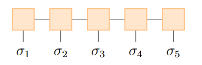
canonical form (normalization) : $A=\Lambda \Gamma$

mps canonical

Example : GHZ or 'cat' state $$ \ket {GHZ} = \frac{1}{\sqrt 2}(\ket{\downarrow}^{\otimes N}+\ket{\uparrow}^{\otimes N}) = \frac{1}{Z}\left(\text{Tr}\left((A^{\uparrow})N\right)\ket{\uparrow}^{\otimes N}+\text{Tr}\left((A^\downarrow)N\right)\ket{\downarrow}^{\otimes N} \right) $$ where $Z$ is a norm and $A^\downarrow_i = A^\downarrow = \begin{bmatrix}1&0\\0&0\end{bmatrix}\quad A^\uparrow_i = A^\uparrow = \begin{bmatrix}0&0\\0&1\end{bmatrix}$

Example : AKLT state

ground state of spin-1 Hamiltonian : $\hat H = \sum_j \hat {\vec S_j}\cdot \hat {\vec S}_{j+1} + \frac{1}{3}\left(\hat{\vec S}_j \cdot \hat{\vec S}_{j+1}\right)^2$

with matrices : $A^+_i = A^+=\sqrt{\frac{2}{3}}\sigma^+ = \begin{bmatrix}0&\sqrt{\frac{2}{3}}\\0&0\end{bmatrix}\quad A^0_i = A^0 =\frac{-1}{\sqrt 3}\sigma^z = \begin{bmatrix}-\frac{1}{\sqrt{3}} & 0 \\0 & \frac{1}{\sqrt 3}\end{bmatrix}\quad A^-_i = A^- = - \sqrt{\frac{2}{3}}\sigma^- \begin{bmatrix}0&0\\-\sqrt{\frac{2}{3}}&0\end{bmatrix}$

the corresponding $\ket +$, $\ket -$ , $\ket 0$ are three states for spin-1 particle not for spin-$\frac{1}{2}$ particle

Notation

$A_i$ : a rank-3 tensor, $A_i\in \mathbb C^{D\times 2\times 2}$, $D$ is the number of basis state for single site.

$A_i^{s_i}$ means when the site $i$ is in state $s_i$, there is a $2\times2$ matrix for product

For translationally symmetric $A_i=A$

$\sigma^+$ : creation / raising operator , $\sigma^+ = \begin{bmatrix}0&0\\1&0\end{bmatrix}$

$\sigma^+ \ket \downarrow = 0$

$\sigma^+ \ket \uparrow =\ket \downarrow$

$\sigma^-$ : annihilation / lowering operator, $\sigma^- = \begin{bmatrix}0&1\\0&0\end{bmatrix}$

$\sigma^- \ket \downarrow = \ket \uparrow$

$\sigma^- \ket \uparrow = 0$

$\ket +$ : for spin-1 , $\ket + = \ket {\uparrow\uparrow}$

$\ket -$ : for spin-1 , $\ket - = \ket{\downarrow\downarrow}$

$\ket 0$ : for spin-1 , $\ket 0 = \frac{1}{\sqrt 2}\left(\ket{\uparrow\downarrow}+\ket{\downarrow\uparrow}\right)$

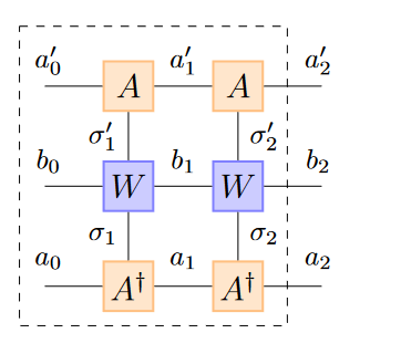
[MPO] Matrix Product Operator : $\hat O = \sum_{\sigma_i,\sigma_i'}\left[W_1^{\sigma_1\sigma_1'}\cdots W_N^{\sigma_N\sigma_N'}\right]\ket{\sigma_1\dots\sigma_N}\bra{\sigma_1'\cdots\sigma_N'}$

mpo

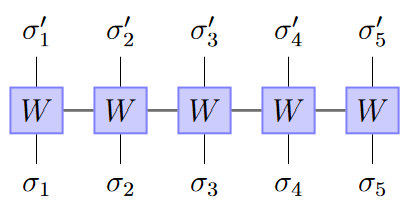
computing $\bra \psi \hat O\ket \psi$ :

mps mpo computation

Example : single site operator

$\hat O_j = I\otimes\cdots\otimes \underbrace{\hat O}_{\text{site}~j}\otimes\cdots\otimes I$

$W_i^{\sigma_i,\sigma_i'}=\bra {\sigma_i}\hat O\ket {\sigma_i'}$

Example : paramagnetic system $\hat H = -\sum_i h\hat S_i^z$

$\hat H = (-h\hat S^z\otimes I\otimes \cdots \otimes I)+\cdots + (I\otimes \cdots\otimes I\otimes -h\hat S^z)$

$W_1 = \begin{bmatrix}-hS^z&I\end{bmatrix}\quad W_i=\begin{bmatrix}I&0\\-hS^z&I\end{bmatrix}\quad W_N=\begin{bmatrix}I\\-hS^z\end{bmatrix}$

Example : Transverse field Ising model $\hat H =-\sum_i \hat S_i^z\hat S_{i+1}^z + h\sum_i\hat S_i^x$

$W_1 = \begin{bmatrix}hS^x&-S^z&I\end{bmatrix}\quad W_i =\begin{bmatrix}I&0&0\\S^z&0&0\\hS^x&-S^z&I\end{bmatrix}\quad W_N = \begin{bmatrix}I\\S^z\\hS^x\end{bmatrix}$

Notation

$W_i$ a rank-4 tensor, $W_i\in \mathbb C^{D\times D\times 2\times 2}$

$W_i^{\sigma_i\sigma_j}$ means for site $i$ when the left state is $\sigma_i$ and right state $\sigma_j$ there is a $2\times2$ matrix for product

[DMRG] Density matrix renormalization group¶

find the ground state that $\underset{\ket \psi}{\text{argmin}}\frac{\bra \psi \hat H \ket \psi}{\braket{\psi}}$

left normalization : $A^\dagger A = I\quad A'=U\Sigma V^\dagger\to A = U$
right normalization : $BB^\dagger = I\quad B'=U\Sigma V^\dagger\to B=V^\dagger$
substitution algorithm : imaginary time evolution, but converge slower

Algorithm

random initialize $\ket \psi$ as right-normalized

build $R_1$

repeat until energy converge $\text{Var}(H)<\epsilon$

right sweep for $l=1,\dots,L-1$

solve eigen value for $M_l$

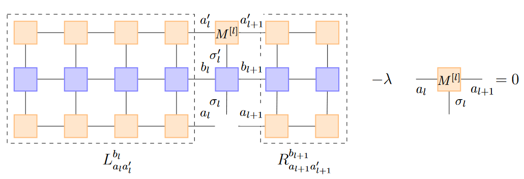
left normalize $M_l$

build $L_l$

Left sweep for $l=L,\dots,2$

solve eigen value for $M_l$

right normalize $M_l$

build $R_l$

[TEBD] Time evolving block decimation¶

TEBD

Algorithm

two site tensor contraction

apply evolution gate

split into single site tensor

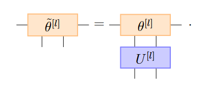
truncation : keep $\chi_{\text{max}}$ eigen value and renormalize $\sum_i\Lambda_ii^2=1$

Computation errors :

truncation error : main error, grows exponentially
Trotter error : can be avoid reducing $\Delta t$ and higher expansion
small eigen value : at step 3 $\Lambda^{-1} A$ and $B\Lambda^{-1}$
imaginary time evolution : canonical form only retrained when $\Delta\tau\to 0$

Further topics¶

Two-dimensional system

converting two dimension system as chain

2D as chain

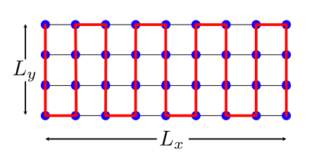
[PEPS] projected entangled pair state

pep

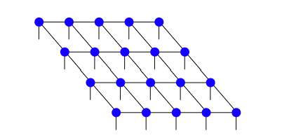
challenging computationally
lack a canonical form

Mixed state and open quantum system dynamics

mixed state unitary time evolution is governed by $\hat H$ : $\partial_t \hat \rho(t)=-i[\hat H,\hat \rho(t)]$
open quantum system : coupled to an environment or bath

which can be described by Lindblad equation : $\partial _t \hat \rho =\hat{\mathcal L}\hat \rho = -i[\hat H,\hat \rho] + \sum_i\gamma_i\left(\hat L_i\hat \rho \hat L_i^\dagger - \frac{1}{2}\{\hat L_i^\dagger\hat L_i,\hat \rho\}\right)$

lindbladian

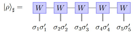
Notation

$\hat L_i$ : jump operator, the system operators directly coupled to the bath, e.g. creation, annilation

$\hat {\mathcal L}$ : Lindbladian, could be considered as a linear operator $\ket {\rho(t)}=e^{-i\hat {\mathcal L}t}\ket{\rho_0}$

Symmetries

schmidt eigenstates belong to a fixed magnetization sector

symmetry schmidt

[TDVP]Time-dependent variational principle

action function : $S=\int_{t_1}^{t_2}\bra {\psi(t)}i\partial_t-\hat H\ket {\psi(t)}\text dt \to \partial_tA_i=-iH_iA_i$
analogue to DMRG algorithm, but better at simulate long-ranged

Quantum Monte Carlo¶

Monte Carlo Basics¶

Monte Carlo

error $\frac{1}{\sqrt N}$

Markov Chain : $P_{XY} = T(X\to Y)A(X\to Y)\quad A(X\to Y) = \text{min}\left\{1,\frac{W(Y)}{W(X)}\right\}$

Ergodicity : $T(X\to Y)>0\quad \forall X,Y$
Normalization : $\sum_Y T(X\to Y)=1$
Reversibility : $T(X\to Y) = T(Y\to X)$, if $T$ not satisfy this, then $A(X\to Y) = \text{min}\left\{1,\frac{W(Y)T(Y\to X)}{W(X)T(X\to Y)}\right\}$

Notation

$T$ : transition probability

$W$ : static distribution

$A$ : accept probability

Classical Ising model¶

symmetry-braking phase transition at a finite temperature $$ H = -\sum_{} J_{ij}\sigma_i\sigma_j - \sum_i h\sigma_i\quad \sigma_i=\pm 1 $$

Notation

$J_{ij}$ : coupling constant

$J_{ij} \ge 0$ : symmetry-broken state

$h_i$ : external field

$<i,j>$ : means $i,j$ are connected

$c$ : cluster, $|c|$ means the number of spins inside a cluster

$\beta$ : inverse temperature, $\beta = \frac{1}{\kappa_B T}$

$m$ : magnetization

Algorithm : Swendsen-Wang

two neighboring parallel spins connected with probability $p=1-e^{-2\beta J}$

cluster labeling. e.g., Hoshen-Kopelman algorithm

measurement : $\langle m^2\rangle_{C'} = \frac{1}{N^2}\sum_c |c|^2$

cluster flipped with probability $\frac{1}{2}$

Algorithm : Wolff

random site

recursive find parallel neighbor add it to the cluster with $p=1-e^{-2\beta J}$

measurement : $\langle m^2\rangle_{C'}=\frac{1}{N}|c_0|$, since only one cluster

flip all spins in the clster

Swendsen-Wang will result in many small clusters in high dimension, but Wolff will result in one large cluster

Quantum spin system thermodynamics¶

\[ \langle \hat m \rangle = \frac{1}{Z}\text{Tr}\left(\hat m e^{-\beta \hat H}\right)=\frac{1}{Z}\sum_C m(C)W(C)\quad Z = \text{Tr}\left(e^{-\beta\hat H}\right)=\sum_C W(C) \]

Notation

$\hat m$ : magnetization

$\beta$ : reverse of temperature $\beta = \frac{1}{\kappa_B T}$

$Z$ : partition sum

$m(C)$ : magnetization of a configuration $C$

$W(C)$ : weight of a configuration $C$

spin-$\frac{1}{2}$ in a magnetic field : $\hat H = -h \hat S^z -\Gamma \hat S^x=\begin{bmatrix}-\frac{h}{2}&-\frac{\Gamma}{2}\\-\frac{\Gamma}{2}&\frac{h}{2}\end{bmatrix}$

Notation

$h$ : longitudinal field

$\Gamma$ : transverse field

Discrete-time path integral : $\beta = \Delta\tau M$

expand to first order $e^{-\Delta \tau \hat H} = \hat U +\mathcal O(\Delta\tau^2)\to Z \approx \text{Tr}\left(\hat U^M\right)$

Notation

$\hat U$ : transfer matrix : $\hat U = I - \Delta \tau \hat H = \begin{bmatrix}1+\frac{\Delta\tau h}{2}&\frac{\Delta\tau\Gamma}{2}\\\frac{\Delta\tau \Gamma}{2}&1-\frac{\Delta \tau h}{2}\end{bmatrix}$

$\Delta \tau$ : discrete time step

$M$ : resolution

$E_0$ : ground energy

Example : 1D classical Ising model (0D transverse field Ising model)

$H = -J\sum_i^M\sigma_i\sigma_{i+1}-h\sum_i \sigma_i$ with periodic boundary condition $\sigma_{M+1}=\sigma_1$

$\beta J = -\frac{1}{2}\text{log}(\Delta \tau \Gamma/2)$ : off diagonal

$\beta h = \text{log}(1+\Delta \tau h/2)$ : diagonal

$\beta E_0 = M\beta J$

Continous-time path integral: $\Delta\tau \to 0$ ???

$d$ -dimensional quantum spin model $\Leftrightarrow$ $d+1$- dimensional classical Ising model

Example : 1D classical Ising model (0D transverse field Ising model)

quantum $XY$ model : $\hat H = -\sum_{<i,j>}\frac{J_{xy}}{2}(\hat S_i^+\hat S_j^- + \hat S_i^-\hat S_j^+)$

spin flip-flops (blue line) proportional to $\beta$ which is a constant not grow bigger as $\Delta \tau \to 0$

spin conservation

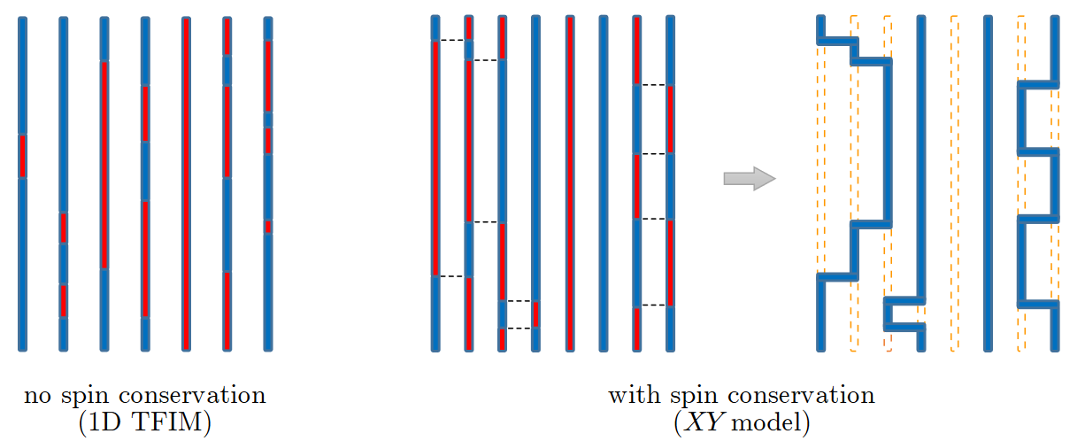
negative sign problem : positive off diagonal lead to negative probabilities

solution : $\langle \hat A\rangle_W = \frac{\sum_C A(C)W(C)}{\sum_C W(C)} = \frac{\sum_C A(C)\text{sign}(W)|W(C)|/\sum_C |W(C)|}{\sum_C \text{sign}(W)|W(C)|/\sum_C|W(C)|}$
error : $\beta\uparrow ,L\uparrow\to \epsilon\uparrow$ error $\epsilon$ increase with inverse temperature $\beta$ and system size $L$

Variational Monte Carlo¶

variational principle : $\ket {\psi(\theta)} = \sum_n \psi_n(\theta)\ket n$

energy expectation(MCMC) : $E_\theta = \frac{\sum_n |\psi_n(\theta)|^2E_1(n)}{\sum_n |\psi_n(\theta)|^2}$

Notation

$E_1(n)$ : local energy $E_1(n)=\sum_m \bra n\hat H\ket m\psi_m(\theta)\psi_n(\theta)$

$G_{kl}$ : metric tensor $G_{kl} = \langle\hat O_k^*\hat O_l\rangle_\theta - \langle \hat O_k^*\rangle_\theta\langle\hat O_l\rangle_\theta$

$O$ : logarithm wave-function derivative $O = \nabla_\theta \psi_n(\theta)/\psi_n(\theta)$

$\hat O = \sum_n O(n)\ket n \bra n$

[SGD]Stochastic Graident Descent : $\theta\gets \theta - \lambda \nabla_\theta E_\theta$

$\nabla_\theta\langle E\rangle_\theta = 2\text{Re}\left\{\sum_n W(n)[E_1(n)-E_\theta]O(n)\right\}$

Stochastic Reconfiguration : $\theta\gets \theta - \Delta \tau G^{-1}\nabla_\theta E_\theta$

to avoid small value inverse : $G' = \sqrt{\beta^2I + G^\dagger G}\quad \beta\in \R$

Jastrow States : $\psi_n(\theta ) = \text{exp}\left(\sum_i a_i\sigma_i + \sum_{<ij>}J_{ij}\sigma_i\sigma_j \right)\quad \theta= \{a,J\}$

wave function form for spin system

[NQS]Neural Quantum States : $\psi_n(\theta)=\text{MLP}(\{\sigma_1,\cdots,\sigma_N\})$

[MFPWF]Mean-field projected wave function : $\ket {\psi(\theta)} = \mathcal P_G \left[\sum_{i,j}\sum_{s,s'}F_{ij}^{ss'}\hat c_{i,s}^\dagger\hat c_{j,s'}^\dagger\right]^{N/2}\ket 0\quad \theta = F_{ij}^{ss'}\in\R^{2N\times 2N}$

$\psi_n(\theta) = (N/2)!\text{Pf}(X)$

represent spin as pesudo-fermions : $\hat S_i^{\{x,y,z\}} = \frac{1}{2}\sum_{ss'}\hat c_{i,s}\sigma_{ss'}^\alpha\hat c_{i,s'}$

Notation

$\mathcal P_G$ : Gutzwilller projection operator

$\hat c_{i,s},\hat c_{i,s}^\dagger$ : fermionic annihlation/creation operator

$s,s'$ : spin of the site, $\uparrow$ or $\downarrow$

$i,j$ : index of the site

Path integrals in quantum statistical mechanics¶

$\rho_{\text{free}}(\vec R,\vec R',\Delta\tau) = \bra {\vec R} e^{-\Delta\tau\hat T}\ket{\vec R'}=\left(\frac{2\pi\hbar^2 \Delta\tau}{m}\right)^{-Nd/2}\text{exp}\left({-\frac{|\vec R-\vec R'|^2}{2\hbar^2\Delta\tau/m}}\right)$

$Z = \int \text d\vec R \rho(\vec R,\vec R)=\int \left(\prod_{j=1}^M \text d\vec R_j\right)\prod_{j=1}^M \left[\left(\frac{2\pi\hbar^2 \Delta \tau}{m}\right)^{-Nd/2}\text{exp}\left(-\frac{\vec R_j-\vec R_{j+1}}{2\hbar^2\Delta\tau/m}-\Delta\tau V(\vec R_j)\right)\right]$

Notation

$\rho_{\text{free}}$ : density matrix of free particles

$Z$ : partition function

$\vec R_j$ : $(\vec r_1,\vec r_2,\cdots,\vec r_N)$ , $N$ particles position at time $j$

$\hat T,\hat V$ : kinetic, potential terms of Hamiltonian $\hat H$, $\hat T = -\frac{\hbar^2}{2m}\partial_x^2$

path sampling method : $A(X\to X' ) = \text{min}\left\{1, \frac{\text{exp}(-m[(\vec r_{j-1}^i - \vec r_j^{i'})^2+(\vec r_j^{i'}-\vec r^i_{j+1})^2]/2\hbar^2\Delta\tau)}{\text{exp}(-m[(\vec r_{j-1}^i-\vec r_j^i)^2+(\vec r_j^i - \vec r_{j+1}^i)^2]/2\hbar^2\Delta \tau)}\cdot \text{exp}(-\Delta \tau[V(\vec R'_j)-V(\vec R_j)])\right\}$

The accept probability of Metropolis algorithm is defined above

$H = \sum_j\sum_i \frac{m}{2(\hbar\Delta \tau)^2}(\vec r_j^i-\vec r_{j+1}^i)^2+\sum_j V(\vec R_j)$

Notation

$\vec r_j^i$ : position of particle $i$ at time $j$

$\vec r_j^{i'}$ : displaced position of particle $i$ at time $j$

$\vec R_j$ : $(\vec r_1,\vec r_2,\cdots,\vec r_N)$ , $N$ particles position at time $j$

$V$ : potential energy, in most cases it's sum of single-particle and two-particle terms : $\hat V = \sum_i^N v_{\text{ext}}(\hat{\vec r}^i) + \sum_{i<j}v(\hat{\vec r}^i -\hat{\vec r}^j)$

Boson symmetry :

$\rho_{\text{Bose}} = \frac{1}{N!}\sum_P \rho(\vec R_1,P\vec R_2, \beta)$

[DMC] Diffusion Monte Carlo¶

diffusion monte carlo

Algorithm

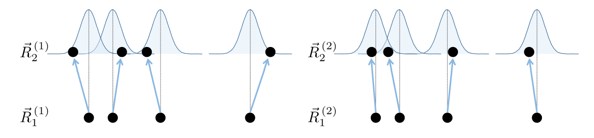
$w_0^\alpha \gets 1,\vec R_0^\alpha \gets \vec R_0$

update loop

$\vec R^\alpha_k \sim \mathcal N(\vec R^\alpha_{k-1},\frac{\Delta \tau}{m})$ : diffusion update

$w_k^\alpha\gets w_{k-1}^\alpha e^{-\frac{\Delta \tau}{2}[V(\vec R_k^\alpha)+V(\vec R^\alpha_{k-1})]}$

clone $\lfloor \frac{w_k^\alpha}{\mathbb E_\alpha [w_k^\alpha]} + r\rfloor$ times for walker $\alpha$

maximum clones $\Leftrightarrow$ $\Delta \tau$ too large
scale $w^\alpha\to\text{exp}(E_t\Delta \tau)w^\alpha$ where $E_t$ is trial energy $V(\vec R)\gets V(\vec R)-E_t$, when $E_t=E_0$ stability will achieve.

Importance sampling : $\vec R_{k-1} \gets \vec R_{k-1}+\frac{\hbar^2\Delta\tau}{2m}\frac{2\nabla\phi_t(\vec R_{k-1})}{\phi(\vec R_{k-1})}$

before update, add a dift : $\vec R_{k-1} \gets \vec R_{k-1}+\frac{\hbar^2\Delta\tau}{2m}\frac{2\nabla\phi_t(\vec R_{k-1})}{\phi(\vec R_{k-1})}$

Notation

$\phi_t$ : trial wavefunction $\phi_t(\vec R)= \prod_{i<j}f_z(|\vec r_i -\vec r_j|)$

$f_z$ : Jastrow factor, two particle coorelations

Fermionic systems : $\phi_{t'}(\vec R)=\phi_t(\vec R)\underset{l,n}{\text{det}}[e^{i\vec k_l\cdot \vec r_n}]$

$\phi_0$ could be negative, when $\phi\to-\phi$ should be applied

Notation

$n$ : particle index

$\vec k_l$ : wave vectors compatible with periodic boundary conditions

Electronic-structure problem¶

Full Hamiltonian of matter¶

\[ \hat H = -\underbrace{\sum_j^{N_e}\frac{\hbar^2}{2m}\nabla^2_{\vec r_j}}_{\hat T_e}- \underbrace{\sum_l^{N_n}\frac{\hbar^2}{2M_l}\nabla^2_{\vec R_l}}_{\hat T_n} + \underbrace{\frac{1}{2}\sum_{i\neq j}^{N_e}\frac{e^2}{|\vec r_i -\vec r_j|}}_{V_{ee}}+\underbrace{\frac{1}{2}\sum_{l\neq m}^{N_n}\frac{Z_lZ_me^2}{|\vec R_l-\vec R_m|}}_{V_{nn}}-\underbrace{\sum_{j=1}^{N_e}\sum_{l=1}^{N_n}\frac{Z_le^2}{|\vec r_j -\vec R_l|}}_{V_{en}}+V_{SO} \]

Adiabatic (Born-Oppenheimer) approximation : $M_l \gg m\quad |\vec R_l-\vec R_m| \ll |\vec r_i - \vec r_j|$ $$ \hat H = \underbrace{\sum_{j=1}^{{N_e}\frac{\hbar}2}{2m}\nabla^2_{\vec r_j}}{\hat T_e} - \underbrace{\sum^{{N_e}\sum_{j=1}}}\frac{Z_le^2}{|\vec r_j - \vec R_l|}{V}}+\underbrace{\frac{1}{2}\sum_{i\neq j^{N_e}\frac{e2}{|\vec r_i-\vec r_j|}}{V $$ }Non-interacing (mean-field) approximation : $\hat H_{\text{sp}} = -\frac{\hbar^2}{2m}\nabla^2_{\vec r}+V_{\text{eff}}(\vec r)$

non-interacting electrons assumption, $V_{en}+V_M + V_{ee}\to V_{\text{eff}}$

Hatree-Fock approximation :

use a Slater determinant for non-interacting system $$ \begin{aligned} \bra \Phi \hat H\ket\Phi &= \underbrace{\sum_{i,\sigma}\int \text d^3 \vec r~\phi_i^{\sigma}(\vec r)[-\frac{\hbar^2}{2m}\nabla2 + V_{en}(\vec r)]\sigma_i^\sigma(\vec r) + V_M}{\hat T_e+ V \ &\begin{drcases} + \sum_{i,j,\sigma,\sigma'}e^2\int \text d^3\vec r~\text d^3\vec r'~\phi_i^{\sigma}}(\vec r)~\phi_j^{\sigma'}(\vec r')\frac{1}{|\vec r-\vec r'|}\phi_i^\sigma(\vec r)\phi_j^{\sigma'}(\vec r')&\text{Hatree interaction} \ % -\sum_{i,j,\sigma}e^2\int \text d^3\vec r~\text d^3\vec r'~\phi_i^{\sigma}(\vec r)~\phi_j^{\sigma*}(\vec r)\frac{1}{|\vec r-\vec r'|}\phi_j^\sigma(\vec r)\phi_i^\sigma(\vec r')&\text{exchange interaction} \end{drcases} V_{ee} \end{aligned} $$ The integration shows that the wave function $\psi$ is defined in the whole space

Notation

$i,j$ : index of the single particle state

$\sigma,\sigma'$ : spin of the electron, $\uparrow$ or $\downarrow$

$\phi_i^\sigma(\vec r)$ : dnotes for particle $i$ of state $\sigma$ , the wave function value at position $\vec r$

Configuration-Interaction : $\ket {\Phi_0} = \left(1+\sum_{i,\mu}\alpha_\mu^i\hat c^\dagger_i\hat c_\mu +\sum_{i<j,\mu<\nu}\alpha_{\mu,\nu}^{ij}\hat c^\dagger_i\hat c^\dagger_j \hat c_\mu \hat c_\nu\right)\ket {\Phi_{\text{HF}}}$

add interations between electrons correctly and allow calculation of excited state

Notation

$\ket {\Phi_{\text{HF}}}$ : Hartree-Fock ground state, which is from the Hartree-Fock approximation, $\ket {\Phi_{\text{HF}}}=\prod_{\mu=1}^N \hat c^\dagger_\mu \ket {\text{nulll}}$

$\hat c^\dagger, \hat c$ : creation / annihilation operator

[DFT] Density functional theory¶

Hohenberg-Kohn Theorem : for electron system $\hat H = \underbrace{-\frac{\hbar^2}{2m}\sum_j\nabla_j^2}_{\hat T_e}+\underbrace{\frac{1}{2}\sum_{i\neq j}\frac{e^2}{|\vec r_i -\vec r_j|}}_{\hat V_{ee}}+\underbrace{\int v_{\text{ext}}(\vec r)n(\vec r)\text d\vec r}_{\hat V_{\text{ext}}}$

Uniqueness : $n_0(\vec r) \Leftrightarrow v_{\text{ext}}(\vec r)$
Variational : $n_0 = \underset{n}{\text{argmin}}~E = \underset{n}{\text{argmin}}\bra\Psi \hat H\ket \Psi$

Notation

$v_{\text{ext}}(\vec r)$ : external potential density

$n_0(\vec r)$ : ground state electron density

$n(\vec r)$ : electron density $\sum_j|\phi_j(\vec r)|^2$

Kohn-Sham solution :

find a non-interacting system that has the same particle density as the interacting one

Algorithm

initial guess $V^0_{\text{eff}}$

solve $\phi_j$ (eigen vector) from KS1 : $\left[-\frac{\hbar^2}{2m_e}\nabla^2+V_{\text{eff}}(\vec r)\right]\phi_j(\vec r) = \varepsilon_j \phi_j(\vec r)$

$n(\vec r)\gets \sum_i |\phi_j(\vec r)|^2$

revise $V_{\text{eff}}$ from KS 2 : $V_{\text{eff}}(\vec r) = \int \text d^3 r'\frac{n(\vec r')}{|\vec r-\vec r'|}+\mu^{\text{XC}}(\vec r)+\nu_{\text{ext}}(\vec r)$

goto 2 if $|V_{\text{eff}}^{\text{new}}-V_{\text{eff}}^{\text{odd}}|\ge \text{threshold}$

Notation

$\mu^{\text{XC}}$ : functional derivative of the exchange-correlation energy, $\mu^{\text{XC}} = \frac{\text d\text E^{\text{XC}}}{\text d n}$

$E^{\text{XC}}$ : exchange-correlation energy, $E^{\text{XC}}=\bra \Phi \hat T\ket \Phi - E_k +\bra \Phi \hat V_{ee}\ket \Phi -E_c$ with approximation (local density approximation) $E^{\text{XC}}\approx \int n(\vec r) \varepsilon^{\text{XC}}(n(\vec r))\text d\vec r=\int n(\vec r)[\varepsilon^X(n(\vec r))+\varepsilon^C(n(\vec r))]\text d\vec r$

uniform electron gas : $\varepsilon(n(\vec r)) = -\frac{3}{4}\left(\frac{3}{\pi}\right)^{1/3}n(\vec r)^{1/3}$

Monte carlo -> interpolation

$E_C$ : Hartree energy $E_C= \frac{1}{2}\int e^2 \frac{n(\vec r)n(\vec r')}{|\vec r-\vec r'|}\text d\vec r\text d \vec r'$

$E_K$ : kinetic energy $E_K = -\frac{\hbar^2}{2m}\sum_j \bra {\phi_j}\nabla^2\ket{\phi_j}$

Basis functions¶

Atoms and molecules

[STO] Slater Type Orbitals : $\psi^i_{nlm}(r,\theta,\phi)\propto r^{n-1}e^{-\xi_ir}Y_{lm}(\theta,\phi)$
two nuclei no closed form
[GTO] Gauss Type Orbitals : $\psi_{nlm}^i(\vec r) \propto x^ly^mz^n e^{-\xi_ir^2}$
gaussian product still gaussian easy to integral

Free electron gas $$ \hat H = - \underbrace{\sum_{i=1}^{{N_e}\frac{\hbar}2}{2m}\nabla^2_{\vec r_i}}{\hat T}+\underbrace{e^2\sum}\frac{1}{|\vec r-\vec r'|}{V $$}

plane waves basis : $\psi_{\vec k}(\vec r) = \text{exp}(-i\vec k\cdot \vec r)$
low temperature : Wigner crystal
better basis will be eigenfunctions of harmonic oscillatiors centered around

Pseudo-potentials

only model outer shell with basis, use pseudo potential to model inner shell since they are not involved in chemical bond

Quantum Computing¶

Quantum Computer¶

quantum gates

one-qubit gate

$X$	$\begin{bmatrix}0&1\\1&0\end{bmatrix}$	$Y$	$\begin{bmatrix}0&-i\\i&0\end{bmatrix}$	$Z$	$\begin{bmatrix}1&0\\0&-1\end{bmatrix}$
name	matrix	name	matrix	name	matrix
$H=\frac{X+Z}{\sqrt 2}$	$\frac{1}{\sqrt 2}\begin{bmatrix}1 & 1\\1&-1\end{bmatrix}$	$T$	$\begin{bmatrix}1&0\\0&e^{i\pi/4}\end{bmatrix}$	$S=T^2$	$\begin{bmatrix}1&0\\0&i\end{bmatrix}$

two-quitbit gate $C(U)=\begin{bmatrix}\begin{matrix}1&0\\0&1\end{matrix}&\begin{matrix}0&0\\0&0\end{matrix}\\\begin{matrix}0&0\\0&0\end{matrix}&U\end{bmatrix}$

measurement : $|\bra{z_1z_2\dots}\ket{\psi}|^2$

repeated $\mathcal O(1000)$ times

errors

coupling to environment $\Rightarrow$ mixed density matrix
gate error
read out measurement error

Representing the Hilbert space¶

Spin-$\frac{1}{2}$ system : directly mapped to a qubit

Fermionic system

Jordan-Wigner Transformation : $\ket \Psi = \ket {n_{N-1},\cdots,n_0}\leftrightarrow \ket {z_{N-1},\cdots,z_0}\quad n_i=z_i$

$\hat c_i \leftrightarrow A_iZ_{i-1}\cdots Z_0\quad \hat c^\dagger_i \leftrightarrow A_i^\dagger Z_{i-1}\cdots Z_0\quad A_i = \frac{(X_i+iY_i)}{2}$

measuring parity requires $\mathcal O(N)$ operators
updating an occupation number requires $\mathcal O(1)$ operators
Parity Encoding : $\ket \Psi = \ket {n_{N-1},\cdots,n_0}\leftrightarrow \ket {z_{N-1},\cdots,z_0}\quad z_i = \left[\sum_{j=0}^in_i\right]\text{mod}~2$

$\hat c_i \leftrightarrow X_{N-1}\cdots X_{i+1}(X_iZ_{i-1}+iY_i)\quad \hat c^\dagger _i \leftrightarrow X_{N-1}\cdots X_{i+1}(X_iZ_{i-1}-iY_i)$

measuring parity requires $\mathcal O(1)$ operators
updating an occupation requires $\mathcal O(N)$ operators
Bravyi-Kitaev : a hypbrid of Parity and Jordan-Wigner

Notation

$n_i$ : fermionic orbitals/site occupation number $n_i\in \{0,1\}$

$\hat c_i, \hat c_i^\dagger$ : creation operator, annihilation operator

Variational quantum solver¶

extract the spectrum of an operator

[QFT] Quantum fourier transform

exact solution
vast number of gate operations

[VQE] Variational Quantum Eigensolver : $\underset{\theta}{\text{min}}\frac{\bra{\Psi(\theta)}\hat H\ket{\Psi(\theta)}}{\bra{\Psi(\theta)}\ket{\Psi(\theta)}}$

quantum computer : expectation evaluation
classical computer : optimization COBYLA (no SGD since no gradient)

[UCC] Unitary Coupled Cluster : $\ket {\Psi(\theta)} = e^{\hat T(\theta)-\hat T^\dagger(\theta)}\ket{\Psi_0}$

a good choice for variational state
huge circuit depth
much depend on the choice of state $\ket{\Phi_0}$

[UCCSD] Unitary Coupled Cluster with Single and Double excitation

$\hat T(\theta) \approx \hat T_1(\theta_1)+\hat T_2(\theta_2)$
$\hat T_1(\theta_1)=\sum_{i,j}\theta_{1,i,j}\hat c^\dagger_i\hat c_j$
$\hat T_2(\theta_2) = \sum_{i,j}\theta_{2,i,j,k,l}\hat c^\dagger_i\hat c^\dagger_k\hat c_j\hat c_l$

Notation

$\hat T(\theta)$ : excitation operator

$\ket {\Psi_0}$ : Hartree-Fock/single Slater detereminant state

\(X\)	\(\begin{bmatrix}0&1\\1&0\end{bmatrix}\)	\(Y\)	\(\begin{bmatrix}0&-i\\i&0\end{bmatrix}\)	\(Z\)	\(\begin{bmatrix}1&0\\0&-1\end{bmatrix}\)
name	matrix	name	matrix	name	matrix
\(H=\frac{X+Z}{\sqrt 2}\)	\(\frac{1}{\sqrt 2}\begin{bmatrix}1 & 1\\1&-1\end{bmatrix}\)	\(T\)	\(\begin{bmatrix}1&0\\0&e^{i\pi/4}\end{bmatrix}\)	\(S=T^2\)	\(\begin{bmatrix}1&0\\0&i\end{bmatrix}\)