NVIDIA Cosmos 平台架构全解¶

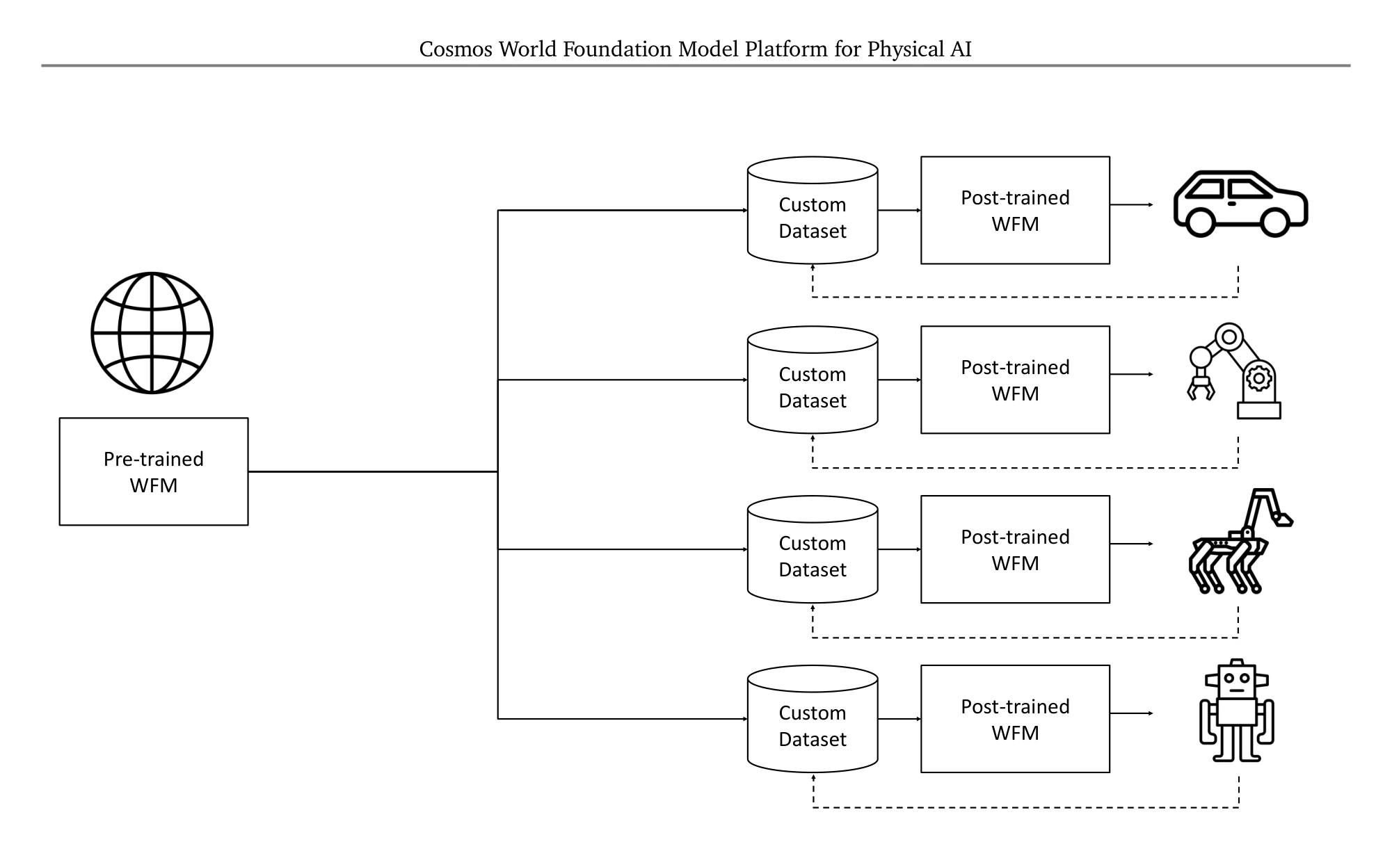
Cosmos WFM Pipeline（原论文 arXiv:2501.03575 Figure 2）

最后更新: 2026-04-14 | 深度调研

Cosmos Tokenizer¶

编码器-解码器架构, 时序因果卷积 + 因果注意力 + 二级小波变换
最大压缩比: 2048x (时序8x × 空间16x16)
PSNR 37.27 (SOTA), 比竞品快2-12x, 压缩量提升8x
连续型(CV)供扩散模型 + 离散型(DV, 64K词汇量)供自回归
12个预训练变体开源

Cosmos-Predict¶

扩散路线(7B/14B): 整流流速度预测, 3D Patchification, AdaLN-LoRA(减36%参数)
自回归路线(4B-13B): 解码器only Transformer, 3D RoPE, 渐进预训练(17→121帧)
Predict2.5: 统一Text/Image/Video2World, 集成Reason1编码器, RL后训练, 30秒生成
训练: 2亿高质量视频片段

Cosmos-Transfer¶

多ControlNet并联: 分割/深度/边缘/人体关键点/LiDAR/HD地图/3D bbox
Transfer2.5(2B): 模型缩小3.5x, 自动驾驶检测精度提升60%
7路相机交叉注意力实现多视角一致性

Cosmos-Reason2¶

基于Qwen3-VL(2B/8B), 256K上下文窗口
三阶段训练: 预训练→SFT(物理AI专项)→RL
Physical AI Bench排行榜第一
56B版本物理常识: 60.2%(超OpenAI o1的59.9%)

训练规模¶

9000万亿tokens, 2000万小时视频
10,000台H100 x 3个月
5阶段数据流水线: 切分→过滤→标注→去重→分片

开源组件¶

全系列模型权重(NVIDIA Open Model License)
Tokenizer/Predict/Transfer/Reason均开源
训练脚本(Apache 2.0), TokenBench评测数据集
专有: 内部VLM标注模型, 原始训练数据集

参考¶

工程实现细节¶

DiT 单块张量流（AdaLN-Zero）¶

AdaLN-Zero 是 DiT 区别于普通 Transformer 的核心：从条件 c（时间步+文本）预测每层的 scale/shift 参数，并用初始化为零的 gate 门控残差。

import torch
import torch.nn as nn

class DiTBlock(nn.Module):
    """
    一个 DiT 块的完整张量流 (Cosmos Predict 采用此架构)

    输入:
      x: (B, N, D)           - token sequence, N = T/t  H/h  W/w
      c: (B, D_cond)         - condition (time embedding + text pooled)
    """
    def __init__(self, d_model=4096, num_heads=32, mlp_ratio=4.0):
        super().__init__()
        self.norm1 = nn.LayerNorm(d_model, elementwise_affine=False, eps=1e-6)
        self.norm2 = nn.LayerNorm(d_model, elementwise_affine=False, eps=1e-6)

        self.attn = nn.MultiheadAttention(d_model, num_heads, batch_first=True)
        self.mlp = nn.Sequential(
            nn.Linear(d_model, int(d_model * mlp_ratio)),
            nn.GELU(approximate='tanh'),
            nn.Linear(int(d_model * mlp_ratio), d_model),
        )

        # AdaLN-Zero: 6 sets of modulation params per block
        # shift/scale/gate for both attention and MLP
        self.adaLN_modulation = nn.Sequential(
            nn.SiLU(),
            nn.Linear(d_model, 6 * d_model, bias=True)
        )
        # 关键初始化: 最后的 Linear 权重+偏置全零
        # 使得早期训练时 gate=0, attention 和 mlp 对输出贡献为 0
        nn.init.zeros_(self.adaLN_modulation[-1].weight)
        nn.init.zeros_(self.adaLN_modulation[-1].bias)

    def forward(self, x, c):
        # x: (B, N, D), c: (B, D)
        # 1. 从条件预测 6 个 modulation 参数
        mod = self.adaLN_modulation(c)                        # (B, 6D)
        shift_msa, scale_msa, gate_msa, \
        shift_mlp, scale_mlp, gate_mlp = mod.chunk(6, dim=1)  # 各 (B, D)

        # 2. Attention 分支: LN → scale+shift → Attn → gate
        x_norm1 = self.norm1(x)                               # (B, N, D)
        x_mod = x_norm1 * (1 + scale_msa.unsqueeze(1)) + shift_msa.unsqueeze(1)
        attn_out, _ = self.attn(x_mod, x_mod, x_mod)          # (B, N, D)
        x = x + gate_msa.unsqueeze(1) * attn_out              # gated residual

        # 3. MLP 分支
        x_norm2 = self.norm2(x)
        x_mod = x_norm2 * (1 + scale_mlp.unsqueeze(1)) + shift_mlp.unsqueeze(1)
        mlp_out = self.mlp(x_mod)
        x = x + gate_mlp.unsqueeze(1) * mlp_out

        return x  # (B, N, D)

# ========== AdaLN-LoRA: 11B → 7B 参数压缩 ==========
# 标准 AdaLN: 每个 block 的 modulation MLP 是 d_model × 6*d_model = 4096 × 24576
# Cosmos 用低秩分解:
class AdaLNLoRA(nn.Module):
    def __init__(self, d_model=4096, lora_rank=64):
        # 共享 Embedding → LoRA down/up projection per block
        self.down = nn.Linear(d_model, lora_rank, bias=False)
        self.up = nn.Linear(lora_rank, 6 * d_model, bias=True)
        nn.init.zeros_(self.up.weight); nn.init.zeros_(self.up.bias)

    def forward(self, c):
        return self.up(self.down(c))

# 参数对比:
# 标准 AdaLN per block: 4096 * 24576 = 100.7M
# AdaLN-LoRA per block: 409664 + 6424576 = 0.26M + 1.57M = 1.83M
# 36 blocks × 节省 ≈ 3.56B 参数!

Rectified Flow Matching 训练与采样¶

# ============ 训练 Loss ============
def flow_matching_loss(model, x0, c):
    """
    x0: (B, T, H, W, C) - 真实数据 (经 VAE/Tokenizer 编码后的 latent)
    c: 条件 (text + ego_dynamics 等)

    核心: 学习速度场 v_θ(x_t, t) 使得插值路径是直线
    """
    B = x0.shape[0]

    # 采样随机噪声和时间
    x1 = torch.randn_like(x0)                     # (B, T, H, W, C)
    t = torch.rand(B, 1, 1, 1, 1).to(x0.device)   # (B, 1, 1, 1, 1)

    # GAIA-2/Cosmos 实际使用双峰 logit-normal:
    # if rand < 0.8: t ~ LogitNormal(0.5, 1.4)
    # else:          t ~ LogitNormal(-3.0, 1.0)
    # 这让训练重点落在中段去噪(μ=0.5)和纯噪声附近(μ=-3.0)

    # 线性插值 (Rectified Flow 的精髓)
    x_t = (1 - t)  x1 + t  x0                   # t=1 → x0, t=0 → x1

    # 目标速度 = x0 - x1 (常数向量!)
    v_target = x0 - x1

    # 预测速度
    v_pred = model(x_t, t.squeeze([-1,-2,-3,-4]), c)

    return F.mse_loss(v_pred, v_target)

# ============ 采样 (Euler ODE) ============
@torch.no_grad()
def sample_flow_matching(model, shape, c, num_steps=50, cfg_scale=4.0):
    """
    Rectified Flow 的 ODE: dx/dt = v_θ(x_t, t)
    Euler 法: x_{t+dt} = x_t + dt * v_θ(x_t, t)
    """
    x = torch.randn(shape).cuda()                  # t=0: 纯噪声
    dt = 1.0 / num_steps

    for step in range(num_steps):
        t_cur = step * dt
        t_tensor = torch.full((shape[0],), t_cur).cuda()

        # Classifier-Free Guidance
        v_cond = model(x, t_tensor, c)             # 条件预测
        v_uncond = model(x, t_tensor, None)        # 无条件预测
        v = v_uncond + cfg_scale * (v_cond - v_uncond)

        x = x + dt * v                             # Euler 一步

    return x  # t=1: 生成样本

# ============ 为什么 Rectified Flow 需要更少步? ============
# DDPM 前向过程: 弯曲扩散路径 → 求解需多步
# Rectified Flow: 直线路径 (v 是常数) → 理论上 1 步就够, 实际 25-50 步足以
#
# 关键洞察: E[x0 - x1 | x_t] 是 noisy target, 模型学到的是条件期望的速度
# 30 次 Euler 迭代 vs DDPM 的 1000 次 ≈ 33× 加速

Cosmos Tokenizer: FSQ 与 3D 因果卷积¶

# ============ 3D 因果卷积 ============
class CausalConv3d(nn.Module):
    """
    保证时序因果性: 当前帧只依赖过去帧, 不看未来
    空间维度正常 padding
    """
    def __init__(self, in_ch, out_ch, kernel=(3,3,3)):
        super().__init__()
        kt, kh, kw = kernel
        self.kt = kt
        # 时间维度 padding 只在前面 (kt-1), 空间正常对称
        self.conv = nn.Conv3d(
            in_ch, out_ch, kernel,
            padding=(0, kh//2, kw//2)  # T 维度 padding=0, 手动 pad 前面
        )

    def forward(self, x):
        # x: (B, C, T, H, W)
        # 前面 pad (kt-1) 个 0, 保证 output[:, :, t] 只依赖 input[:, :, <=t]
        x = F.pad(x, (0, 0, 0, 0, self.kt - 1, 0))
        return self.conv(x)

# ============ FSQ (Finite Scalar Quantization) ============
class FSQ(nn.Module):
    """
    替代 VQ-VAE 的无码本量化方法
    将连续向量的每一维量化到预定义的几个 level 上
    """
    def __init__(self, levels=[8, 5, 5, 5, 6, 4]):
        super().__init__()
        self.levels = levels
        self.num_dim = len(levels)
        # 词表大小 = ∏ levels = 85556*4 = 24,000 (Cosmos 用 64,000)
        self.codebook_size = 1
        for l in levels: self.codebook_size *= l

    def forward(self, z):
        """
        z: (B, D, T, H, W) with D = num_dim
        """
        # Step 1: bound into [-1, 1]
        z = torch.tanh(z)

        # Step 2: 每维映射到 [-(L-1)/2, (L-1)/2] 并四舍五入
        out = []
        for i, L in enumerate(self.levels):
            z_i = z[:, i:i+1]
            half_l = (L - 1) / 2
            z_scaled = z_i * half_l
            # 直通估计器 (STE): forward 取 round, backward 用恒等梯度
            z_quant = z_scaled + (z_scaled.round() - z_scaled).detach()
            out.append(z_quant / half_l)        # 归一化回 [-1, 1]

        z_q = torch.cat(out, dim=1)
        return z_q

    def to_index(self, z_q):
        """从量化向量得到单个 codebook 索引"""
        idx = 0
        multiplier = 1
        for i, L in enumerate(self.levels):
            # z_q[:,i] ∈ {-1, ..., 1} 有 L 个值
            half_l = (L - 1) / 2
            bucket = ((z_q[:, i] * half_l) + half_l).long()  # 0..L-1
            idx = idx + bucket * multiplier
            multiplier *= L
        return idx  # (B, T, H, W)

# ============ 为什么 FSQ > VQ-VAE ============
# VQ-VAE 痛点:
#   1. 码本崩溃 (大量码字从未被用)
#   2. 需要 commitment loss, EMA codebook update 等 tricks
# FSQ 优势:
#   1. 无码本, 不会崩溃
#   2. 无辅助 loss
#   3. 训练更稳定, 重建质量相当或更好

Tokenizer 整体架构与压缩比¶

Grouped Query Attention 与 KV Cache¶

# ============ GQA 实现 ============
class GroupedQueryAttention(nn.Module):
    """
    Dreamer V4 / Cosmos AR 使用 GQA: 16 Q heads, 4 KV heads
    相比 MHA: KV 内存降至 1/4
    相比 MQA: 性能损失少, 灵活性高
    """
    def __init__(self, d_model=4096, num_q_heads=16, num_kv_heads=4):
        super().__init__()
        self.num_q_heads = num_q_heads
        self.num_kv_heads = num_kv_heads
        self.head_dim = d_model // num_q_heads  # 256
        self.group_size = num_q_heads // num_kv_heads  # 4 Q heads share 1 KV head

        # Q 全大小, KV 小 4 倍
        self.W_q = nn.Linear(d_model, num_q_heads * self.head_dim, bias=False)
        self.W_k = nn.Linear(d_model, num_kv_heads * self.head_dim, bias=False)
        self.W_v = nn.Linear(d_model, num_kv_heads * self.head_dim, bias=False)
        self.W_o = nn.Linear(num_q_heads * self.head_dim, d_model, bias=False)

    def forward(self, x, kv_cache=None, causal=True):
        B, N, D = x.shape

        Q = self.W_q(x).reshape(B, N, self.num_q_heads, self.head_dim)   # (B, N, 16, 256)
        K = self.W_k(x).reshape(B, N, self.num_kv_heads, self.head_dim)  # (B, N, 4, 256)
        V = self.W_v(x).reshape(B, N, self.num_kv_heads, self.head_dim)  # (B, N, 4, 256)

        # KV Cache: 增量生成时只处理新 token
        if kv_cache is not None:
            K_cached, V_cached = kv_cache                # (B, N_past, 4, 256)
            K = torch.cat([K_cached, K], dim=1)          # (B, N_past+N_new, 4, 256)
            V = torch.cat([V_cached, V], dim=1)

        # Repeat KV 以匹配 Q 的 heads
        # Flash Attention 2 内部优化: 不实际 repeat, 用广播
        K_rep = K.repeat_interleave(self.group_size, dim=2)  # (B, N, 16, 256)
        V_rep = V.repeat_interleave(self.group_size, dim=2)

        # (B, heads, N, head_dim)
        Q = Q.transpose(1, 2)
        K_rep = K_rep.transpose(1, 2)
        V_rep = V_rep.transpose(1, 2)

        # Scaled Dot-Product Attention (用 flash attention 加速)
        out = F.scaled_dot_product_attention(Q, K_rep, V_rep, is_causal=causal)
        out = out.transpose(1, 2).reshape(B, N, -1)

        new_cache = (K, V) if kv_cache is not None else None
        return self.W_o(out), new_cache

# ============ KV Cache 内存节省 ============
# 标准 MHA: 16 heads × seq_len × head_dim × 2 (K+V) × 2 bytes (bf16)
# seq_len=8192, 16 heads, head_dim=256:
#   MHA Cache: 16 × 8192 × 256 × 2 × 2 = 134 MB per layer
#   GQA Cache:  4 × 8192 × 256 × 2 × 2 =  33 MB per layer (4× 节省)
# 36 层: MHA 4.8 GB vs GQA 1.2 GB — 关键于长上下文自回归生成

Cosmos EDM 预条件化（数值稳定核心）¶

# ============ EDM (Elucidating Diffusion Models) ============
# 不同 σ 下网络的输入/输出尺度差异巨大
# 若不预条件化, 在 σ=80 (纯噪声) vs σ=0.002 (几乎干净) 时网络行为完全不同
# EDM 的 4 个预条件化系数让网络在所有 σ 下看到 ~O(1) 的输入输出

def edm_denoise(model, x, sigma, sigma_data=0.5):
    """
    EDM 预条件化去噪函数
    x: 带噪声的输入
    sigma: 噪声水平 (scalar 或 per-sample)
    sigma_data: 数据标准差 (超参数, Cosmos ~0.5)
    """
    # 预条件化系数
    c_in  = 1.0 / torch.sqrt(sigma2 + sigma_data2)   # 归一化输入
    c_noise = sigma.log() / 4                             # 输入网络的 σ 表示
    c_skip = sigma_data2 / (sigma2 + sigma_data2)   # skip 连接权重
    c_out  = sigma * sigma_data / torch.sqrt(sigma2 + sigma_data2)  # 输出缩放

    # 网络预测在规约空间
    F_theta = model(c_in * x, c_noise)                    # (B, ...) 目标是 ~N(0,I)

    # 反预条件化: 还原为原始尺度的去噪预测
    D = c_skip  x + c_out  F_theta
    return D  # 预测的 clean x

# ============ EDM Sampling (Heun 二阶求解器) ============
@torch.no_grad()
def edm_sample(model, shape, num_steps=30, sigma_min=0.002, sigma_max=80, rho=7):
    """
    EDM σ 调度: σ_i = (σ_max^{1/ρ} + i/(N-1) * (σ_min^{1/ρ} - σ_max^{1/ρ}))^ρ
    ρ=7 让步长在高 σ 处密集, 低 σ 处稀疏 — 更好利用算力
    """
    # 非均匀 σ schedule
    step_indices = torch.arange(num_steps)
    t = (sigma_max(1/rho) + step_indices / (num_steps - 1) *
         (sigma_min(1/rho) - sigma_max(1/rho)))  rho
    t = torch.cat([t, torch.zeros_like(t[:1])])  # 末尾加 0

    x = torch.randn(shape) * sigma_max
    for i in range(num_steps):
        t_cur, t_next = t[i], t[i+1]

        # 去噪
        denoised = edm_denoise(model, x, t_cur.expand(shape[0]))

        # Heun 二阶修正 (除最后一步)
        d_cur = (x - denoised) / t_cur
        x_next = x + (t_next - t_cur) * d_cur

        if t_next > 0:
            denoised_next = edm_denoise(model, x_next, t_next.expand(shape[0]))
            d_next = (x_next - denoised_next) / t_next
            x = x + (t_next - t_cur)  0.5  (d_cur + d_next)  # 平均斜率
        else:
            x = x_next

    return x

Cosmos 14B 训练并行化策略¶

训练规模¶

训练配置: 9000 万亿 tokens / 10,000 × H100 / 3 个月 ≈ 1e22 FLOPs 总计算量。每个 batch 大约 5-10M tokens，总步数约 9-18 亿步（分阶段）。

关键数学公式¶

DiT AdaLN-Zero 调制¶

从条件 c 预测 6 组参数（scale/shift/gate 各 2 对）：

\([\gamma_1,\beta_1,\alpha_1,\gamma_2,\beta_2,\alpha_2] = \operatorname{MLP}(c)\)

Attention 分支：\(x \leftarrow x + \alpha_1\cdot\operatorname{Attn}\!\left(\gamma_1\cdot\operatorname{LN}(x) + \beta_1\right)\)

MLP 分支：\(x \leftarrow x + \alpha_2\cdot\operatorname{MLP}\!\left(\gamma_2\cdot\operatorname{LN}(x) + \beta_2\right)\)

最后一层 MLP 权重初始化为零 → 早期训练 \(\alpha \approx 0\)，残差分支“冷启动”。

AdaLN-LoRA（11B→7B 关键）¶

标准 AdaLN 每层参数 O(d²)；LoRA 分解为低秩：

\(\operatorname{MLP}(c) = W_{\text{up}}\,W_{\text{down}}\,c,\quad W_{\text{down}}\in\mathbb{R}^{r\times d},\ W_{\text{up}}\in\mathbb{R}^{6d\times r}\)

\(r=64\) → 每层 100.7M 降到 1.83M，36 层共节省约 3.56B 参数。

Rectified Flow / Flow Matching¶

线性插值路径：\(x_t = (1-t)\,x_1 + t\,x_0,\quad t\in[0,1]\)

目标速度（常数！）：\(v^*_t = x_0 - x_1\)

训练目标：\(\mathcal{L}_{\text{FM}} = \mathbb{E}_{t,x_0,x_1}\!\left[\|v_\theta(x_t,t) - (x_0-x_1)\|_2^2\right]\)

Euler 采样：\(x_{t+dt} = x_t + dt\cdot v_\theta(x_t,t)\)

Classifier-Free Guidance¶

\(\tilde v_\theta(x_t,t,c) = v_\theta(x_t,t,\varnothing) + w\cdot\left[v_\theta(x_t,t,c) - v_\theta(x_t,t,\varnothing)\right]\)

等效于隐式分类器引导 \(\nabla \log p(c|x)\)。\(w \in [2, 20]\)，小 w 多样性高、大 w 条件保真度高。

EDM 预条件化（4 个系数）¶

输入缩放：\(c_{\text{in}}(\sigma) = 1/\sqrt{\sigma^2 + \sigma_d^2}\)

输出缩放：\(c_{\text{out}}(\sigma) = \sigma\cdot\sigma_d / \sqrt{\sigma^2 + \sigma_d^2}\)

Skip 权重：\(c_{\text{skip}}(\sigma) = \sigma_d^2 / (\sigma^2 + \sigma_d^2)\)

σ 编码：\(c_{\text{noise}}(\sigma) = \ln(\sigma)/4\)

去噪函数：

\(D(x;\sigma) = c_{\text{skip}}(\sigma)\cdot x + c_{\text{out}}(\sigma)\cdot F_\theta\!\left(c_{\text{in}}(\sigma)\cdot x,\ c_{\text{noise}}(\sigma)\right)\)

Karras σ Schedule¶

\(\sigma_i = \left(\sigma_{\max}^{1/\rho} + \frac{i}{N-1}\left(\sigma_{\min}^{1/\rho} - \sigma_{\max}^{1/\rho}\right)\right)^\rho\)

\(\rho=7\) → 高 \(\sigma\) 处步长密集、低 \(\sigma\) 处稀疏，更好利用算力。

EDM Heun 二阶求解器¶

当前斜率：\(d_i = (x_i - D(x_i,\sigma_i))/\sigma_i\)

试探步：\(x_{i+1}^{\text{tmp}} = x_i + (\sigma_{i+1}-\sigma_i)\cdot d_i\)

Heun 修正：\(x_{i+1} = x_i + (\sigma_{i+1}-\sigma_i)\cdot\frac{1}{2}\left(d_i + d_{i+1}\right)\)

FSQ（有限标量量化）¶

对每一维独立量化到 L 个 level（无需 codebook）：

\(z_q^{(i)} = \frac{1}{L_i/2}\cdot\operatorname{round}\!\left(\frac{L_i}{2}\cdot\tanh(z^{(i)})\right)\)

词表大小 = \(\prod L_i\)。Cosmos 用 [8,5,5,5,6,4] → 24,000 词；实际部署 64,000。

GQA 注意力¶

Q 头数 H_q，KV 头数 H_{kv}，groupsize g = H_q/H_{kv}：

\(\operatorname{GQA}(Q,K,V) = \operatorname{Softmax}\!\left(\frac{Q\,\operatorname{repeat}(K)^\top}{\sqrt{d_h}}\right)\operatorname{repeat}(V)\)

Dreamer V4 / Cosmos AR 用 16:4 = 4×，KV cache 内存降至 \(1/4\)。

Code 引用索引与可信度¶

✓=官方代码直接移植, △=基于论文描述重构, ⚠=推测填充 ——

注: 所有 "✓" 级代码的完整版本请参考对应 GitHub repo；本文的 PyTorch 伪代码经过简化以突出核心逻辑。

↑ 上级 · 02 技术架构与核心方法