NumPDENumerical Method for Partial Differential Equation

---

professor : Ralf Hiptmair

author: walkerchi

---

Basic Mathematic

Theorem

• Gauss's Theorem : \(\int_\Omega \text{div}~\textbf{j}~\text{d}x = \int_{\partial \Omega}\textbf{j}\cdot\textbf{n}~\text{d}S(x)\)
• Green's first formula : \(\int_{\Omega}\textbf{j}\cdot\ v~\text{d}x = - \int_{\Omega}\nabla \cdot ~\textbf{j}~v~\text{d}x +\int_{\partial \Omega}\textbf{j}\cdot \textbf{n}~v~\text{d}S\)
• General product rule : \(\text{div}(\textbf{j}~v) = v~\text{div}\textbf{j} + \textbf{j}\cdot \nabla v\)

Notation

• \(\textbf{n} : \partial\Omega \to \R^d\) exterior unit normal vector field on \(\partial \Omega\)
• \(\textbf j\in \R^d\) : flux vector, e.g. velocity field
• \(\Omega\) : interior domain
• \(\partial \Omega\) : domain boundary

Definition

• \(\text{inf}\{x\}\in \R^d\) : infinite set , the lower bound
• \(\text{sup}\{x\} \in \R^d\) : super set, the upper bound

Sobolev Space & Norm

• \(L^2\) norm : \(\Vert v\Vert_{L^2} = \sqrt{\int_\Omega \Vert v(x) \Vert^2 dx}\)

• \(C_{pw}^0(\Omega) \subset L^2(\Omega)\)

• \(H^1(\Omega)\) seminorm : \(\vert v\vert_{H^1} = \sqrt{\int_{\Omega}\Vert\nabla v\Vert^2 dx} = \Vert \nabla v\Vert _{L^2}\)

• \(H^1_0(\Omega)\) denotes the boundary \(\partial \Omega\) is \(0\)

• \(C_{pw}^0(\Omega)\not\subset H^1(\Omega) \quad C_{pw}^1(\Omega)\subset H^1(\Omega)\)

• \(H^1(\Omega)\) norm : \(\Vert v\Vert_{H^1} = \sqrt{\Vert v\Vert_{L^2}^2 + \vert v\vert_{H^1}^2}\)

• Multiplicative trace inequality : \(\Vert u \Vert^2 _{L^2 (\partial \Omega)} \le C\Vert u\Vert_{L^2(\Omega)} \cdot \Vert u\Vert_{H^1(\Omega)}\quad \exists C = C(\Omega) > 0\)

• \(H^m(\Omega)\) norm : \(\Vert v\Vert_{H^m} = \underset{\boldsymbol \alpha \in \N^d,|\boldsymbol \alpha|=m}{\sum}\int_\Omega \vert \text{D}^{\boldsymbol\alpha} u\vert^2\text d\boldsymbol x\)

• \(\Vert\cdot\Vert_{\text a}\) energy norm : \(\Vert v\Vert_{\text a}=\sqrt{a(v,v)}\)

Boundary

• Dirichelet boundary (essential boundary) : \(u = g\quad u\in \partial \Omega\)
• Neumann boundary (natural boundary) : \(\frac{\partial u}{\partial \textbf{n}} = \textbf{j}\cdot \textbf{n}= -h\quad u\in \partial \Omega\)
• compatibility condition : \(-\int_{\partial \Omega}h~dS = \int_{\Omega} fdx\) for the existence of Neumann problem
• variational form example : \(\int_\Omega \kappa(\boldsymbol x)\nabla u\cdot \nabla v~d\boldsymbol x + \int_{\partial\Omega}\Psi(u)~v~d\mathcal S = \int_{\Omega}fv~d\boldsymbol x\quad\begin{matrix}u\in H^1(\Omega)\\\forall v\in H^1(\Omega)\end{matrix}\)
• Radiation boundary : \(\frac{\partial u}{\partial \textbf{n}} = \Psi(u) \quad u \in\partial \Omega\)

Notation

• \(\textbf{n} : \partial\Omega \to \R^d\) exterior unit normal vector field on \(\partial \Omega\)
• \(\textbf j\in \R^d\) : flux vector, e.g. velocity field
• \(\Omega\) : interior domain
• \(\partial \Omega\) : domain boundary

Forms

• Minimization problem : \(u = \underset{v}{\text{argmin}}~J(v) =\underset{v}{\text{argmin}}~\frac{1}{2}\text{a}(v,v) - \ell(v) =\underset{v}{\text{argmin}}~\frac{1}{2}\Vert v\Vert_\text{a} - \ell(v)\)
• LVP (Generalized) Linear variational problem : \(\text{a}(u,v) = \ell(v) \quad \begin{matrix}u\in \hat V_0 \\ \forall v\in V_0\end{matrix}\), \(\hat V_0\) is the trial space, \(V_0\) is the test space
• example :
• BVP Boundary value problem
• DVP Discrete variational problem : \(\text{a}(u_h,v_h) = \ell(v_h)\quad \begin{matrix}u_h\in V_{0,h}\\\forall v_h \in V_{0,h}\end{matrix}\) where \(u\) is test space, \(v\) is trial space
• IVP Initial boundary problem : \(\dot {\textbf y} = f(t,\textbf y)\quad \textbf y(t_0)=\textbf y_0\)
• Strong form : a partial differential equation (PDE)
• example : \(-\nabla^2 u = f\)
• Weak form : add test space and integrate in domain to the strong form
• example : \(-\nabla^2 u = f \to \int_\Omega \nabla u \cdot \nabla v~\text d x - \int_{\partial\Omega} \nabla u \cdot\boldsymbol n~v~\text d\mathcal S = \int_\Omega f~v~\text dx\)

---

FEM Finite Element Method

Galerkin Discretization

\[ a(u_h,v_h) = \ell(v_h) \Leftrightarrow \textbf{A}\vec \mu = \vec \phi \]

Notation

• \(\textbf{A}\) Galerkin matrix (stiffness matrix) : \(\textbf{A} = \left[\text{a}(b_h^k,b_h^j)\right]^N_{j,k=1}\in \R^{N\times N}\)
• \(\textbf{A}\) is symmetric and positive definite
• \(\vec \phi\) : Right hand side vector (load vector) : \(\vec \phi = \left[\ell(b_h^j)\right]_{j=1}^N\in \R^N\)
• \(\vec \mu\) : Coefficient vector : \(\vec \mu =[\mu_1,\cdots,\mu_h]^\top\in\R^N\), \(u_h = \sum_{k=1}^N\mu_kb_h^k\) where \(b_h^k\in\mathfrak B\) is basis function

Basis Function

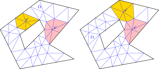
• degree of freedom : basis function \(b_h^k\in\mathfrak{B}_h\)

• change of basis : \(\tilde{\mathfrak{B}_h} = \textbf{S}\mathfrak{B}_h\to \tilde{\textbf{A}} = \textbf S\textbf A\textbf S^\top\quad \tilde{\vec\phi}=\textbf{S}\vec\phi\quad \tilde{\vec \mu} = S^{-T}\vec \mu\)

• support : \(\text{supp}(f) = \{x\in\Omega,f(x)\neq 0\}\)

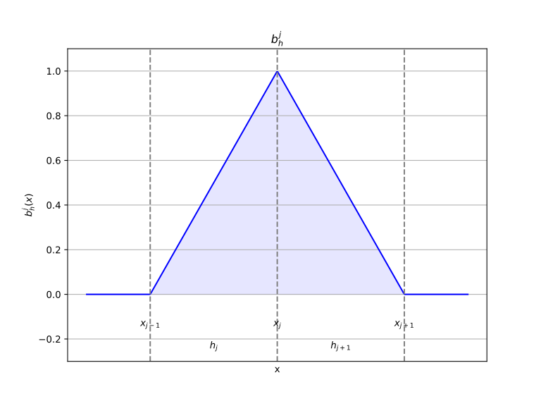
Example 1 : Tent Function 1D

tent function : \(b_h^j(x) = \begin{cases}(x-x_{j-1})/h_j&x_{j-1}\le x\le x_j\\(x_{j+1}-x)/h_{j+1}&x_j\le x\le x_{j+1}\\0&\text{otherwise}\end{cases}\)

 Example 2 : Triangle Barycentric cooridnate

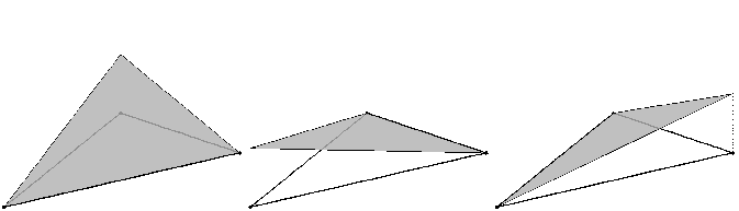
tent function : \(b_h^i(x_j) = \begin{cases}1&i=j\\0&\text{else} \end{cases}\)

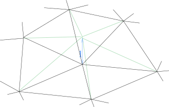
barycentric coordinate function : \(\lambda_i = \alpha_i +\boldsymbol \beta^i \cdot \boldsymbol x \quad \alpha\in\R,\boldsymbol \beta\in\R^3\)

\(a_i^j\) : the \(i\)th component of the \(j\)th point in the triangle element

How to get \(\alpha\) and \(\boldsymbol \beta\) ?

1. solve the linear system $$ \begin{bmatrix} 1&a_1^1&a_21\ 1&a_1^2&a_22\ 1&a_1^3&a_23 \end{bmatrix} \begin{bmatrix} \alpha_1&\alpha_2&\alpha_3\ \beta_1^1&\beta_12&\beta_1^3\ \beta_2^1&\beta_22&\beta_2^3 \end{bmatrix} = I_3 $$

2. compute directly $$ \lambda_1 = \frac{1}{2|K|}\left(\boldsymbol x-\boldsymbol a_K^2\right) \begin{bmatrix} a_2^2 - a_2^3\ a_1^3-a_12 \end{bmatrix} \quad \lambda_2 = \frac{1}{2|K|}\left(\boldsymbol x-\boldsymbol a_K^3\right) \begin{bmatrix} a_2^3 - a_2^1\ a_1^1-a_13 \end{bmatrix} \quad \lambda_3 = \frac{1}{2|K|}\left(\boldsymbol x-\boldsymbol a_K^1\right) \begin{bmatrix} a_2^1 - a_2^2\ a_1^2-a_11 \end{bmatrix} $$

Quadrature

\[ \int_a^b \psi(t)dt \approx \sum_{j=1}^m \omega_j^m \psi(\zeta_j^m) \]

Notation

• \(\omega_j^m\) : quadrature weights
• \(\zeta_j^m\) : quadrature nodes

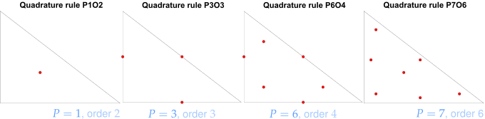
Example : Triangle quadrature

\(K = \text{convex}\left\{\begin{bmatrix}0\\0\end{bmatrix},\begin{bmatrix}1\\0\end{bmatrix},\begin{bmatrix}0\\1\end{bmatrix}\right\}\) : triangle element

• P1O2 : \(\omega=\left\{1\right\}\)， \(\zeta = \left\{\begin{bmatrix}\frac{1}{3}\\\frac{1}{3}\end{bmatrix}\right\}\)
• P3O3 : \(\omega = \left\{\frac{1}{3},\frac{1}{3},\frac{1}{3}\right\}\), \(\zeta = \left\{\begin{bmatrix}\frac{1}{2}\\0\end{bmatrix},\begin{bmatrix}0\\\frac{1}{2}\end{bmatrix},\begin{bmatrix}\frac{1}{2}\\\frac{1}{2}\end{bmatrix}\right\}\)

Stiffness Matrix

\[ [A_K]_{ij} = \text{a}(b_h^i,b_h^j) \]

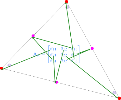
Example : Triangle Element Stiffness Matrix $$ a(\lambda_i,\lambda_j) = \int \nabla\lambda_j(x)\cdot\nabla\lambda_i(x)~dx \ \Rightarrow \textbf{A}_K = |K|\begin{bmatrix}\beta_1^1&\beta_12&\beta_1^3\\beta_21&\beta_2^2&\beta_23\end{bmatrix}^\top \begin{bmatrix}\beta_1^1&\beta_12&\beta_1^3\\beta_21&\beta_2^2&\beta_23\end{bmatrix} $$

Eigen::Matrix<double, 2, 3> gradbarycoordinates(const TriGeo_t& vertices){
    // a -> beta
    Eigen::Matrix<double,  3, 3> X;
    X.block<3,1>(0,0) = Eigen::Vector3d::Ones();
    X.block<3,2>(0,1) = vertices.transpose();
    return X.inverse().block<2,3>(1,0);
}

Eigen::Matrix3d ElementMatrix_Lapl_LFE(const TriGeo_t& V){
    // a -> A
    // TriGeo_t Matrix[n_dim, n_basis] n_dim = 2 n_basis = 3
    double area = 0.5 * std::abs((V(0,1) - V(0,0)) * (V(1,2) - V(1,1)) - 
                                  (V(0,2) - V(0,1)) * （V(1,1) - V(1,0)));
    Eigen::Matrix<double, 2, 3> X = gradbarycoordinates(V);
    return area * X.transpose() * X;
}

Load Vector

\[ [\vec \phi]_j = \ell(b_h^j) \]

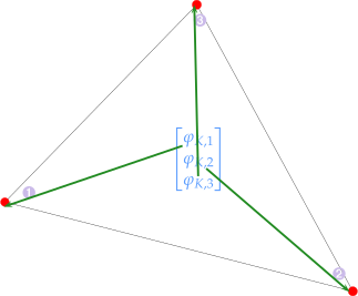
Example : Triangle Element Load Vector $$ \ell(b_h^j) = \int f(b_h^j(x))~dx \\Rightarrow \vec \phi _K = \frac{|K|}{3}\begin{bmatrix}f(a^1)&f(a2)&f(a^{3)\end{bmatrix}}\top $$

typedef function<double(const Eigen::Vector2d &)> FHandle_t;
Eigen::Vector3d localLoadLFE(const t_TriGeo&V, const FHandle_t& FHandle){
    // a -> phi
    // TriGeo_t Matrix[n_dim, n_basis] n_dim = 2 n_basis = 3
    double area = 0.5 * std::abs((V(0,1) - V(0,0)) * (V(1,2) - V(1,1)) - 
                                  (V(0,2) - V(0,1)) * （V(1,1) - V(1,0)));
    Eigen::Vector3d philoc = Eigen::Vector3d::Zero();
    for(int i = 0; i < 3; i ++) philoc(i) = FHandle(V.row(i));
    philoc *= area / 3.0;
    return philoc;
}

---

Assemble

\[ \textbf A_{K} \to \textbf A_\mathcal M\quad \forall K\in \mathcal M \]

construct the global stiffness matrix/load vector using element stiffness matrix/load vector

Stiffness Matrix

• Edge $$ \textbf{A}{ij}=\text{a}\left(b^j,b_{h|K_1}i\right)+ \text{a}\left( b_{h|K_2}^j,b_{h|K_2}i\right) \quad \forall i\neq j $$

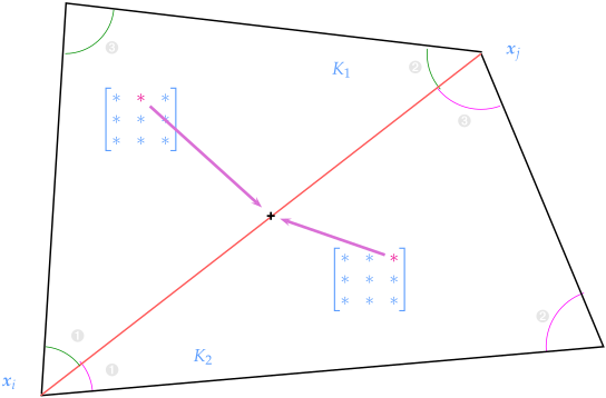
• Node $$ \textbf{A}{ii} = \sum}\text{a}\left(b_{h|K_j^i,b_{h|K_j}i\right) $$

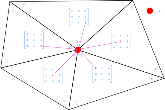
Example : code for stiffness matrix assemble

Eigen::SparseMatrix<double> assembleGalMatLFE(const TriaMesh2D& Mesh, 
                                              const LocalMatrixHandle_t getElementMatrix){
    int N = Mesh._nodecoords.rows(); // Mesh._nodecoords Matrix[n_nodes, n_dim] 
    int M = Mesh._elments.rows();    // Mesh._elements Matrix[n_elements, n_basis]
      Eigen::SparseMatrix<double> A(N,N);
    for(int i = 0; i < M; i++){
        Eigen::Vector3i dofhk = Mesh._elements.row(i); 
        TriGeo_t V; // [n_dim, n_basis] n_dim = 2, n_basis = 3
        for(int j = 0; j < 3; j++)V.col(j) =  Mesh._nodecoords.row(dofhk(j)).transpose();
        Eigen::Matrix3d Ak = getElementMatrix(V);
        for(int j = 0; j < 3; j++)
            for(int k = 0; k < 3; k++)
                A.coeffRef(dofhk(j), dofhk(k)) += Ak(j, k);
    }
    A.makeCompresssed(); // coo to csr
    return A;
}

**LehrFEM++ Example **

computeGalerkinMat : \(\int_\Omega \alpha(x)\nabla u\cdot \nabla v +\gamma(x)~u~v~\text d x + \int_{\partial \Omega}\beta~u~v~\text d\mathcal S = \int_\Omega f~v~\text d x\)

• \(\textbf M=\int_\Omega \rho~u~v~\text dx\)

auto zero_mf = lf::uscalfe::MeshFunctionGlobal([](Eigen::Vector2d)->double{return 0.0;});
auto one_mf = lf::uscalfe::MeshFunctionGlobal([](Eigen::Vector2d)->double{return 1.0});
auto rho_mf = lf::uscalfe::MeshFunctionGlobal(rho);
lf::assemble::COOMatrix<double> M_COO = computeGalerkinMat(fe_space_p, zero_mf, rho_mf, zero_mf);
Eigen::SparseMatrix<double> M = M.makeSparse(); // coo to csr

ReactionDiffusionElementMatrixProvider : \(\text{a}(u,v) = \int_{\Omega} \alpha(x)\nabla u\cdot\nabla v +\gamma(x)~u~v~\text{d}x\)

• \(\textbf M =\int_\Omega u~v~\text dx\)

auto zero_mf = lf::mesh::utils::MeshFunctionConstant(0.0);
auto one_mf = lf::mesh::utils::MeshFunctionConstant(1.0);
lf::uscalfe::ReactionDiffusionElementMatrixProvider M_locmat_builder(fe_space , zero_mf , one_mf);
lf::assemble::COOMatrix<double> M_COO(N_dofs, N_dofs);
//assemble on cell
lf::assemble::AssembleMatrixLocally(0, dofh, dofh, M_locmat_builder,  M_COO); 

• \(\textbf A = \int_{\Omega} \nabla u\nabla v~\text d x\)

auto zero_mf = lf::mesh::utils::MeshFunctionConstant(0.0);
auto one_mf = lf::mesh::utils::MeshFunctionConstant(1.0);
lf::uscalfe::ReactionDiffusionElementMatrixProvider A_locmat_builder(fe_space , one_mf , zero_mf); 
lf::assemble::COOMatrix<double> A_COO(N_dofs, N_dofs);
//assemble on cell
lf::assemble::AssembleMatrixLocally(0, dofh, dofh, A_locmat_builder,  A_COO); 

MassEdgeMatrixProvider : \(\text{a} = \int_{\partial \Omega}\gamma(x)~u~v~\text dx\)

• \(\textbf B = \int_{\partial \Omega} u~v~\text dx\)

auto one_mf = lf::mesh::utils::MeshFunctionConstant(1.0);
lf::mesh::utils::CodimMeshDataset<bool>  bd_flags{ lf::mesh::utils::flagEntitiesOnBoundary(fe_space->Mesh(), 1)
}; // 1  means edge, 0 means triangle
lf::uscalfe::MassEdgeMatrixProvider B_locmat_builder(fe_space_p, one_mf, bd_flags);
lf::assemble::COOMatrix<double> B_COO(N_dofs, N_dofs);
//assemble on edge
lf::assemble::AssembleMatrixLocally(1, dofh, dofh, B_locmat_builder,  B_COO); 

Load Vector

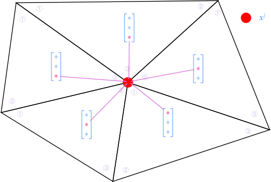
Example : code for load vector assemble

typedef function<double(const Eigen::Vector2d&)> FHandle_t;
typedef function<Eigen::Vector3d(const TriGeo_t&, FHandle_t)> LocalVectorHandle_t;
Eigen::VectorXd assemLoad_FLE(const TriaMesh2D& Mesh,
                             const LocalVectorHandle_t& getElementVector,
                             const FHandler_t& FHandle){
    int N = Mesh._nodecoords.rows(); // Mesh._nodecoords Matrix[n_nodes, n_dim]
    int M = Mesh._elments.rows();    // Mesh._elements Matrix[n_elements, n_basis]
    Eigen::VectorXd phi = Eigen::VectorXd::Zero(N); 
    for(int  i = 0; i < M; i++){
        Eigen::Vector3i dofhk = Mesh._elements.row(i);
        TriGeo_t V; // [n_dim, n_basis] n_dim = 2, n_basis = 3
        for(int j = 0; j < 3; j++)V.col(j) =  Mesh._nodecoords.row(dofhk(j)).transpose();
        Eigen::Vector3d philoc = getElementVector(V, FHandle);
        for(int j = 0; j < 3; j++) phi(dofhk(j)) += philoc(j);
    }
    return phi;
}

Transformation

\[ K = \Phi_K(\hat K) = \textbf F_k \hat K+\tau \Rightarrow |K| =|\hat K| |\text{det} \textbf F_k| \]

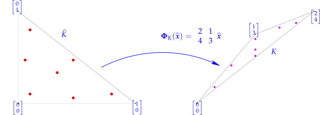
Notation

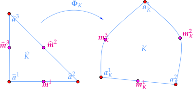
• \(K/\hat K\) : transformed/origin element
• \(\Phi_K\) : transformation for element \(K\), \((\Phi^*u)(x)=\Phi(u(\hat x))\Rightarrow (\nabla_{\hat x}(\Phi^* u))(\hat x) = (\text{D}\Phi(\hat x))^\top\underbrace{(\nabla_x u)\Phi(\hat x)}_{=\Phi^*(\nabla u)(\hat x)}\)

To apply the transformation, following rules are used :

• quadrature : \(\omega_\ell^K = \underbrace{\sqrt{\text{det}(\text{D}\Phi(\hat \zeta_\ell)^\top \text{D}\Phi(\hat \zeta_{\ell}))}}_{\text{\textcolor{yellow}{Gramian determinant}}}\hat\omega_\ell \quad \zeta_\ell^K = \Phi_K(\hat \zeta_\ell)\)
• \(f(x)\to f(\Phi(\hat \zeta))\)
• \(u(x)\to \hat b (\hat \zeta)\)
• \(\nabla u(x)\to \left(\text{D} \Phi(\hat\zeta)\right)^{-\top}\nabla\hat b(\hat \zeta)\)

Example

• \(\text a(u,v) = \int \alpha(x)\nabla u(x)\cdot \nabla v(x)~\text{d}x\) $ {[A_K]}{ij} = \sum\Phi(\hat \zeta_\ell)|$}^P\hat\omega_\ell \alpha\left(\Phi(\hat \zeta_\ell)\right)\left(\left(\text{D}\Phi(\hat\zeta_\ell)\right)^{-\top}\nabla \hat b^i(\hat \zeta_\ell)\right)\cdot\left(\left(\text{D}\Phi(\hat \zeta_\ell)\right)^{-\top}\nabla \hat b^j(\hat \zeta_\ell)\right)~|\text{det D

• \(\ell(v) = \int f(x)~\text{d}x\) $ {[\vec \phi_K]i} = \sum\Phi_K(\hat\zeta_\ell)|$ }^P\hat \omega_\ell f\left(\Phi_K(\hat \zeta_\ell)\right)\hat b^i(\hat \zeta_\ell)~|\text{det D

LehrFEM++

const lf::uscalfe::FeLagrangeO2Tria<double> ref_fe;
const lf::quad::QuadRule qr{lf::quad::make_TriaQR_P6O4};
const lf::geometry::Geometry *geo = cell.Geometry();
const Eigen::VectorXd dets(geo->IntegrationElement(qr.Points()));
const Eigen::VectorXd JinvT(geo->JacobianInverseGramian(qr.Points()));
const Eigen::MatrixXd val_ref_lsf = ref_fe.EvalReferenceShapeFunctions(qr.Points());
const Eigen::MatrixXd grad_ref_lsf = ref_fe.GradientsReferenceShapeFunctions(qr.Points());

• \(\begin{bmatrix}\hat\zeta_1,\cdots,\hat\zeta_m\end{bmatrix}\) : qr.Points()
• \(\hat b^j\) : val_ref_lsf(j, l)
• \(\nabla \hat b^j(\hat \zeta_\ell)\) : grad_ref_lsf.block(j, 2*l, 1, 2).transpose()
• \(\textbf{D}\Phi_K(\hat \zeta_\ell)^{-\top}\) : JinvT.block(0, 2*l, 2, 2)
• \(\text{det D}\Phi_K(\hat \zeta_\ell)\) : dets[l]

Lagrangian FEM

\(\mathcal S_p^0(\mathcal M)\) : \(p\)-th Lagrangian finite element space, \(C^0\) continuity, \(p\) is the degree of polynomials

• Multivariate polynomials : \(\mathcal P_p(\R^d) = \{\boldsymbol x\in\R^d\to \sum_{\boldsymbol \alpha\in \N_0^d,|\boldsymbol \alpha|\le p}c_{\boldsymbol \alpha}\boldsymbol x^{\boldsymbol\alpha},c_{\boldsymbol\alpha}\in \R\}\)
• example : \(\mathcal P_2(\R^2) = \text{Span}\{1,x_1,x_2,x_1^2,x_2^2,x_1,x_2\}\)
• dimension : \(\text{dim} \mathcal P_p(\R^d)=\left(\begin{matrix}d+p\\p\end{matrix}\right)\)
• Tensor product polynomials : \(\mathcal Q(\R^d) = \text{Span}\{x\to p_1(x_1)\cdots p_d(x_d),~p_i\in\mathcal P_p(\R),~i=1,\dots,d\}\)
• example : \(\mathcal Q_2(\R^2) = \text{Span}\{1,x_1,x_2,x_1x_2,x_1^2,x_1^2x_2,x_1^2x_2^2,x_1x_2^2,x_2^2\}\)
• dimension : \(\text{dim}\mathcal Q_p(\R^d) = (p+1)^d\quad \forall p\in\N_0,d\in\N\)

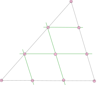
Example : High order triangle element

• Triangle P2

$$ \begin{matrix} b_K^1 = (2\lambda_1 - 1)&b_K^2 = (2\lambda_2 - 1)\lambda_2 & b_K^3 = (2\lambda_3-1)\lambda_3 \ b_K^4 = 4\lambda_1\lambda_2 & b_K^5 = 4\lambda_2\lambda_3 & b_K^6 = 4\lambda_1\lambda_3 \end{matrix} $$

• Triangle P3

• Triangle P\(p\) $$ b_K^i = \sum_{\boldsymbol \alpha\in\N^3_0,|\boldsymbol\alpha|\le p} \kappa_{\boldsymbol\alpha}\lambda_1^{{\alpha_1}\lambda_2} $$ }\lambda_3^{\alpha_3

---

Boundary

Essential boundary (condense)

\[ u = g\quad u\in\partial\Omega\Leftrightarrow \vec \mu_{\partial }=\vec \gamma \]

$$ \begin{bmatrix} \textbf A_0&\textbf A_{0\partial}\ \textbf A_{0\partial}^\top & A_{\partial\partial} \end{bmatrix} \begin{bmatrix} \vec \mu_0\\vec\gamma \end{bmatrix} = \begin{bmatrix} \vec \phi\ * \end{bmatrix} \Leftrightarrow A_0\vec \mu_0 = \vec\phi - A_{0\partial}\vec\gamma $$

LehrFEM++

• FixFlaggedSolutionComponents $$ \text A=\begin{bmatrix} \textbf A_{00}&\textbf A_{0\partial}\ \textbf A_{\partial 0}&\textbf A_{\partial\partial} \end{bmatrix}, \textbf b = \begin{bmatrix} \textbf b_{0}\ \textbf b_{\partial} \end{bmatrix} \ \textbf A\textbf x =\textbf b \Leftrightarrow \begin{bmatrix} \textbf A_{00}&0\ 0&\textbf I \end{bmatrix} \begin{bmatrix} \textbf x\ \hat{\textbf x} \end{bmatrix} = \begin{bmatrix} \textbf b_0 - \textbf A_{0\partial}\hat{\textbf x}\ \hat{\textbf{x}} \end{bmatrix} $$

lf::assemble::FixFlaggedSolutionComponents<double>(
    [&](lf::assemble::gdof_idx_t idx) -> std::pair<bool,double>{
        // if node is boundary, return 0
        const lf::mesh::Entity &node{dofh.Entity(idx)};
        return {bd_flags(node), 0.0}; 
    }
    A, phi);

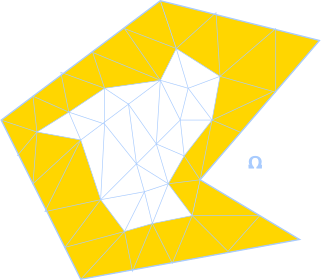
boundary approximation

Convergence and Accuracy

Notation

\(h_\mathcal M\) : mesh width \(h_\mathcal M = \text{max}\{\text{diam}~K:K\in \mathcal M\}\) \(\text{diam} ~K=\text{max}~\{|\textbf p - \textbf q|:\textbf p,\textbf q\in K\}\)

Types of Convergence :

• algebratic convergence : \(\Vert u -u_N\Vert = \mathcal O(N^{-\alpha})\quad\alpha >0\)
• exponential convergence : \(\Vert u -u_N\Vert = \mathcal O(\text{exp}(-\gamma N^\delta))\quad \gamma,\delta >0\)

Concept :

• Shape Regularity : \(\rho_K = \frac{h_K^d}{|K|}\quad \rho_\mathcal M = \underset{K\in M}{\text{max}}~\rho_K\quad h_K = \text{diam}(K)\)

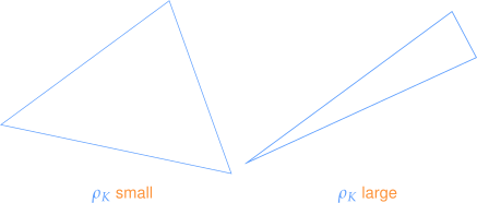
• \(\text{diam}(K)\) : the longest distance between two points in element \(K\)

• \(\rho_{K/\mathcal M}\) : shape regularity for element \(K\) / mesh \(\mathcal M\)

• Variational Crime : instead of solve exact varational problem \(\text{a}(u_h,v_h) = \ell(v_h)\), we solve perturbed varational problem \(\text{a}(\tilde u_h,v_h)=\ell(v_h)\)

Error Estimation

• \(H^1\) norm : \(\underset{v_h\in \mathcal S_p^0(\mathcal M)}{\text{inf}} \Vert u- v_h\Vert_{H^1(\Omega)}\le \underbrace{C\left(\frac{h_\mathcal M}{p}\right)^{\text{min}\{p+1, k\}-1}\Vert u \Vert_{ H^k(\Omega)}}_{C'N^{-\frac{\text{min}\{p,k-1\}}{d}} \Vert u\Vert_{H^k(\Omega)}}\)
• \(\Vert u-\text{l}_p u\Vert _{H^1(\Omega)} \le Ch_\mathcal M^{\text{min}\{p+1,k\}-1}\Vert u\Vert_{H^k(\Omega)}\), \(\text{l}_p\) is the \(p\)-th order interpolation

• \(L^2\) norm : \(\Vert u-v_h\Vert _{L^2(\Omega)/L^\infty(\Omega)} = \mathcal O(h_\mathcal M^{p+1})\)

• \(\Vert u-\text{l}_p u\Vert _{L^2(\Omega)} \le Ch_\mathcal M^{\text{min}\{p+1,k\}}\Vert u\Vert_{H^k(\Omega)}\)

• example : \(\Vert u-\text{l}_1 u\Vert_{L^2(\Omega)}\le \sqrt{\frac{3}{8}}h_\mathcal M^2 |u|_{H^2(\Omega)}\)
• \(H^1\) seminorm : \(\vert u-v_h\vert _{H^1(\Omega)} = \mathcal O(h_\mathcal M^p)\)
• example : \(\vert u-\text{l}_1 u\vert_{H^1(\Omega)}\le \sqrt{\frac{3}{24}}\rho_\mathcal M h_\mathcal M|u|_{H^2(\Omega)}\)

Example

\(-\nabla u = f\quad u\in H^1\)

• linear Lagrangian \(p=1\) \(\mathcal S_1^0\)
• \(|u-u_h|_{H^1(\Omega)} = \mathcal O(h_\mathcal M) = \mathcal O(N^{-\frac{1}{2}})\)
• \(|\vert u-u_h\Vert_{L^2(\Omega)} = \mathcal O(h_\mathcal M^2) = \mathcal O(N^{-1})\)
• \(\Vert u-u_h \Vert _{H^1(\Omega)} = \mathcal O(N^{-\frac{1}{3}})\)
• quadratuic Lagrangian \(p=2\) \(\mathcal S_2^0\)
• \(|u-u_h|_{H^1(\Omega)} = \mathcal O(h_\mathcal M^2) = \mathcal O(N^{-1})\)
• \(\Vert u-u_h \Vert_{L^2} = \mathcal O(h_\mathcal M^3) = \mathcal O(N^{-\frac{3}{2}})\)
• \(\Vert u-u_h\Vert_{H^1(\Omega)} = \mathcal O(N^{-\frac{1}{3}})\)

Nonlinear BVP

Linearizing fixed-point iteration

Example

• \(\int_{\Omega} \textbf A(x,\nabla u)\nabla u\cdot \nabla v + c(u)uv~\text{d}x = \int_\Omega f(x)v ~\text{d} x\)

\(\int_\Omega \textbf A(x,\nabla u^{(k)})\nabla u^{(k+1)}\cdot \nabla v + c(u^{(k)})u^{(k+1)}(x)v(x)\text{d} x = \int_\Omega f(x)v~\text{d}x\)

Newton's method

\[ \begin{aligned} &\text{a}(u^{(k)},v) + \text{D}_u\text{a}(u^{(k)},v)w = 0 \\ &\text{D}_u\text{a}(u^{(k)},v) = \underset{t\to 0 }{\text{lim}}\frac{\text{a}(u+tw,v)-a(u,v)}{t} \\ &u^{(k+1)} = u^{(k)} + w \end{aligned} \]

Example

• \(\text{a}(u,v)=\int_\Omega \sigma(x)\textbf A(\nabla u)\nabla u \cdot \nabla v~\text{d}x\)

\(\begin{aligned} \text{D}_u \text a(u,v)w &= \underset{t\to 0}{\text{lim}}\frac{\int_{\Omega}\sigma(x)\textbf A(\nabla u + t\nabla w)(\nabla u + t\nabla w) \cdot \nabla v~\text{d}x - a(u,v)}{t} \\ &= \underset{t\to 0}{\text{lim}}\frac{\int_{\Omega}\sigma(x)\left(\textbf A(\nabla u)+ t\text{D}\textbf A(\nabla u)\nabla w\right)(\nabla u + t\nabla w) \cdot \nabla v~\text{d}x}{t} \\ &= \int_\Omega \textbf A(\nabla u) \nabla w\cdot \nabla v + (\text D\textbf A(\nabla u)\nabla w)\nabla u \cdot \nabla v~\text{d}x \end{aligned}\)

---

Time Evolution

Notation

• \(\dot u = \frac{\partial u}{\partial t}\)
• \(\ddot u = \frac{\partial^2 u}{\partial t^2}\)

Linear

\[ \textbf M\frac{\text d \vec \mu(t)}{\text dt} + \textbf A\vec \mu(t) = \vec \phi(t) \]

Notation

• \(\textbf M\in \R^{N\times N}\) : mass matrix \(\textbf M_{ij}=\text{m}(b_h^j,b_h^i)\)
• \(\textbf{A} \in \R^{N\times N}\) : stiffness matrix \(\textbf A_{ij} = \text{a}(b_h^j,b_h^i)\)
• \(\vec \phi \in \R^N\) : load vector \(\vec\phi_i(t) = \ell(t)(b_h^i)\)

Example : heat equation $$ \underbrace{\int_\Omega \rho(\boldsymbol x)\dot u(\boldsymbol x)~\text{d}\boldsymbol x}{\text m(\dot u,v)}+\underbrace{\int\Omega\kappa(\boldsymbol x)\nabla u(t)\cdot\nabla v~\text{d}\boldsymbol x}{\text a(u,v)} = \underbrace{\int\Omega f(\boldsymbol x,t)v~\text{d}\boldsymbol x}_{\ell(t)(v)} $$

Runge-Kutta

\[ \dot{\textbf u} = \textbf f(t,\textbf u) \]

\[ \textbf M\dot{\vec \mu} + \textbf A\vec \mu(t) = \vec \phi(t) \Rightarrow \dot{\vec \mu} = \underbrace{\textbf M^{-1}(\vec\phi(t)-\textbf A\vec \mu(t))}_{\textbf f(t,\vec \mu)} $$ **<font color="orange">$\textcolor{orange}{s}$-stage Runge-Kutta single step method</font>** $$ \textbf k_i =\textbf f(t+c_i\tau, \textbf u +\tau \sum_{j=1}^s a_{ij}\textbf k_j)\quad \Psi^{t,t+\tau}\textbf u = \textbf u+\tau\sum_{i=1}^s b_i \textbf k_i $$ **<font color="orange">Butcher schemes</font>** $$ \begin{array}{c|c} \textbf c & \mathfrak A \\ \hline &\textbf b^\top \end{array} \quad = \quad \begin{array}{c|ccc} c_1 & a_{11} & \cdots & a_{1s}\\ \vdots & \vdots & \ddots & \vdots \\ c_s & a_{s1} & \cdots & a_{ss}\\\hline & b_1 & \cdots & b_s \end{array} \qquad \textbf c, \textbf b \in \R^s,\mathfrak A\in \R^{s\times s} \]

Example

• explicit (forward) Euler : \(\begin{array}{c|c}0&0\\\hline&1\end{array}\)
• \(\Psi^{t,t+\tau}\textbf u \approx \textbf u + \tau \textbf f(t,\textbf u)\)
• implicit (backward) Euler : \(\begin{array}{c|c}1&1\\\hline&1\end{array}\)
• \(\Psi^{t,t+\tau}\textbf u \approx \textbf w\quad \textbf w=\textbf u+\tau\textbf f(t+\tau,\textbf w)\)
• implicit midpoint rule : \(\begin{array}{c|c}\frac{1}{2}&\frac{1}{2}\\\hline&1\end{array}\)
• \(\Psi^{t,t+\tau}\textbf u \approx \textbf w\quad \textbf w = \textbf u +\tau \textbf f(t+\frac{\tau}{2},\frac{\textbf w+\textbf u}{2})\)

Diagonalization $$ \textbf T^\top\textbf M\textbf T = \textbf I\quad \textbf A\textbf T = \textbf M\textbf T\textbf D\quad \textbf D=\text{diag}\begin{bmatrix}\lambda_1,\cdots,\lambda_N\end{bmatrix} $$

\[ \textbf M \frac{\text d\vec\mu}{\text dt}+\textbf A\vec \mu = 0\Leftrightarrow\dot {\vec\eta} = -\textbf D\vec \eta\quad \vec\eta = \textbf T^\top \textbf M\vec\mu \]

Behavior of generalized eigenvalues $$ \frac{1}{\text{diam}(\Omega)^2}\le \lambda_{min}\le C\quad\lambda_{\text{max}}\ge Ch_\mathcal M^{-2} $$

• \(\lambda_{\text{min}}\) not depend on \(h_\mathcal M\)
• \(\lambda_{\text{max}}\) propotional to \(h_\mathcal M^{-2}\)

Stability $$ \mathcal S(z) = 1+z\textbf b^\top(\textbf I - z\mathfrak A)^{-1}\textbf 1 = \frac{\text{det}(\textbf I-z\mathfrak A+z\textbf 1\textbf b^\top)}{\text{det} (\textbf I-z\mathfrak A)}\quad z\in \mathbb C $$

\(\text{L}(\pi)\)-stability :

• \(|\mathcal S(z)| < 1\quad \forall z<0\)
• \(\underset{z\in\R\to-\infty}{\text{lim}}\mathcal S(z)=0\)

Convergence $$ \sqrt{\tau\sum_{j=1}^M|u-u_h|_{H1}^2}\le C(h_\mathcal M^p+\tauq) $$ - \(p\) is the degree of Lagrangian finite element - \(q\) is the order of single step method - \(\tau\) is the timestep

Second Order

\[ \textbf M\ddot {\vec\mu(t)} +\textbf A\vec \mu(t) = \vec \phi(t) \]

Example : wave equation $$ \underbrace{\int_\Omega\rho(\boldsymbol x)\cdot \ddot u(\boldsymbol x,t)~v(\boldsymbol x)~\text{d}\boldsymbol x}{=\text{m}(\ddot u,v)} + \underbrace{\int\Omega \sigma(\boldsymbol x)\nabla u (\boldsymbol x,t)\cdot\nabla v(\boldsymbol x)~\text{d}\boldsymbol x}_{\text a(u,v)} = 0 $$

conservation of total energy : \(\frac{1}{2}\text{m}(\dot u,\dot u)+\frac{1}{2}\text{a}(u,u) = \text{const}\)

Crank-Nicolson

\[ \textbf M\frac{\vec \mu^{(j+1)}-2\vec \mu^{(j)}+\vec \mu^{(j-1)}}{\tau^2} = -\frac{1}{4}\textbf A\left(\vec \mu^{(j-1)}+2\vec \mu^{(i)}+\vec \mu^{(j+1)}\right) + \frac{1}{2}\left(\vec\phi(t_j - \frac{\tau}{2})+\vec\phi(t_j +\frac{\tau}{2})\right) $$ ### Störmer-Verlet $$ \textbf M\frac{\vec \mu^{(j+1)}-2\vec \mu^{(j)}+\vec \mu^{(j-1)}}{\tau^2} = -\textbf A\vec \mu^{(j)} +\vec\phi(t_j) $$ ### Leapfrog $$ \begin{aligned} \textbf M\frac{\vec \nu^{(j+\frac{1}{2})}-\vec \nu^{(j-\frac{1}{2})}}{\tau} &= -\textbf A\vec \mu^{(j)} + \vec\phi(t_j) \\ \frac{\vec \mu^{(j+1)}-\vec \mu^{(j)}}{\tau} &= \vec\nu^{(j+\frac{1}{2})} \end{aligned} \]

\[ \begin{aligned} \sqrt{\tau\sum_{j=1}^M\Vert u-u_h\Vert^2_{H^1}}&\le C(h_\mathcal M^p + \tau^2) \\ \sqrt{\tau\sum_{j=1}^M\Vert u-u_h\Vert^2_{L^2}}&\le C(h_\mathcal M^{p+1} + \tau^2) \end{aligned} \]

stability for leapfrog timestepping entails : \(\tau\le \mathcal O(h_\mathcal M)\)

Method of Lines

discrete variables other than time, then solve the equation as ODE

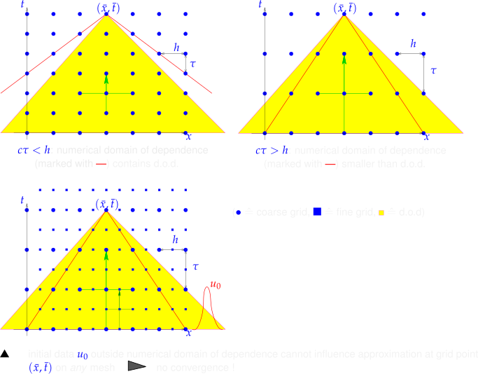
Courant-Fridrichs-Lewy(CFL) condition

maximum speed of propagation : \(s= \text{sup}\{|f'(\zeta)|:\text{inf}~u_0(x)\le \zeta\le \text{sup}~u_0(x)\}\)

minimum timestep : \(\tau \le \frac{h}{s}\)

DoD Domain of Dependency $$ \text{CFL-condition}\Leftrightarrow \text{analytical DoD}\subset \text{numerical DoD} $$

Example : Störmer-Verlet timestepping

---

Convection Diffusion

Heat conduction in a fluid

• CDE (Convection-Diffusion Equation) : \(\underbrace{-\nabla\cdot(\kappa \nabla u(\boldsymbol x))}_{\text{diffusive term(2nd order)}}+\underbrace{\nabla\cdot (\rho\textbf v(\boldsymbol x)u(\boldsymbol x))}_{\text{convective term(1st order)}} = f\)
• Incompressible CDE : \(\underbrace{-\kappa\nabla^2 u}_{\text{diffusive term(2nd order)}} + \underbrace{\rho\textbf v\cdot \nabla u}_{\text{convective term(1st order)}} = f\)
• Time-Depdent(Transient) Heat Flow : \(\frac{\partial (\rho u)}{\partial t} -\kappa\nabla^2u+\rho \textbf v(\boldsymbol x,t)\cdot \nabla u =f(\boldsymbol x,t)\)
• Transport Equation : \(\frac{\partial u}{\partial t} +\textbf v(\boldsymbol x,t)\cdot\nabla u = f(\boldsymbol x)\)

Notation

• \(u\in \R\) : temperature
• \(\textbf v\in \R^d\) : fluid velocity

Maximumm principle $$ \begin{aligned} -\nabla^2 u +\textbf v\cdot\nabla u &\ge 0 \Rightarrow \underset{x\in\partial\Omega}{\text{min}}_{u(x)=\underset{x\in\Omega}{\text{min}}}u(x) \ -\nabla^2 u +\textbf v\cdot\nabla u &\le 0 \Rightarrow \underset{x\in\partial\Omega}{\text{max}}_{u(x)=\underset{x\in\Omega}{\text{max}}}u(x) \end{aligned} $$ Boundary

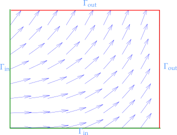
• inflow boundary : \(\Gamma_{\text{in}} = \{x\in\partial\Omega, \textbf v(\boldsymbol x)\cdot \boldsymbol n(\boldsymbol x) < 0\}\)
• outflow boundary : \(\Gamma_{\text{out}} = \{x\in\partial\Omega, \textbf v(\boldsymbol x)\cdot \boldsymbol n(\boldsymbol x) > 0\}\)

Method of Lines

discretized \(d-1\) dimension $$ \frac{\partial u }{\partial t} - \epsilon \nabla^2u +\textbf v(\boldsymbol x, t)\cdot \nabla u = f \ \Downarrow \ \textbf M \frac{\text d\vec \mu }{\text d t}(t) + \epsilon \textbf A\vec \mu(t) + \textbf B(t)\vec\mu(t) =\vec\phi (t) $$

Notation

• \(\vec \mu(t)\in \R^N\) : approximation of \(u_h\)
• \(\textbf M\in\R^{N\times N}\) : mass matrix
• \(\textbf A\in \R^{N\times N}\) : Galerkin matirx
• \(\textbf B(t)\in \R^{N\times N}\) : time-dependent matrix for convection term
• \(\vec \phi(t)\in\R^N\) : load function \(f\) and boundary \(g\)

Upwind

$$ -\epsilon \nabla^2 u + \textbf v\cdot \nabla u = f $$ for very small \(\kappa/\epsilon\) spurious oscillation is observed

• upwind quadrature \(\zeta\to \underset{\delta\to 0}{\text{lim}}~\zeta - \delta \textbf v(\zeta)\)

• convergence : \(\Vert u-u_h\Vert_{L^2} = \mathcal O(h_M)\)

• streamline-diffusion method : \(\epsilon \to \epsilon\textbf I + \delta_K \textbf v_K \textbf v_K^\top\)

• consistency (SUPG stremaline upwind/petrov galerkin method) : $$ \int_\Omega \nabla u\cdot\nabla w+(\textbf v(x)\cdot\nabla u)w~\text d \boldsymbol x + \underbrace{\sum_{K\in\mathcal M}\delta_K\int_K(-\epsilon\nabla^2 u +\textbf v\cdot \nabla u -f)\cdot(\textbf v\cdot \nabla w)\text d\boldsymbol x}{\text{stabilization term}} = \int\Omega fw\text d\boldsymbol x $$

• convergence : \(\Vert u-u_h\Vert_{L^2} = \mathcal O(h_\mathcal M^2)\)

other methods :

• forward differential : \(|\epsilon h^{-1}|\ge 1\) $$ \frac{\text d u}{\text d x}|{x=x_i} = \frac{u $$}-u_{i}}{h

• backward differential : \(\epsilon \ge 0, h>0\) $$ \frac{\text d u}{\text d x}|{x=x_i} = \frac{u_i-u $$}}{h

Split-Step method

Strang Splitting

\[ \dot {\textbf y} = g(t,\textbf y)+r(t,\textbf y) \]

1. \(\tilde {\textbf y} = \textbf z(t_{j-1},\frac{1}{2}\tau)\quad \dot{\textbf z}=g(t,\textbf z)\quad \textbf z(t_{j-1})=y^{(j-1)}\)
2. \(\hat{\textbf y} = \textbf w(t_j)\quad \dot {\textbf w} = \textbf r(t,\textbf w)\quad \textbf w(t_{j-1})=\tilde y\)
3. \(\textbf y^{(j)} = \textbf z(t_j)\quad \dot {\textbf z}=\textbf g(t,\textbf z)\quad \textbf z(t_{j-1}+\frac{1}{2}\tau)=\hat{\textbf y}\)

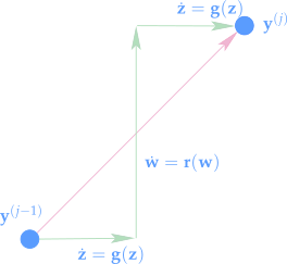
accuracy order: second order

Leap-frog : combine 1 and 3

---

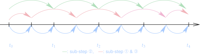
Conservation

Characteristics

characteristic curve : \(\Gamma := (\gamma(\tau),\tau)\), usually \(x=\gamma(\tau)\) $$ \frac{\text d}{\text d\tau}\gamma(\tau) = f'\left(u\left(\gamma(\tau),\gamma\right)\right) $$

Reimann problem

\[ u_0 = \begin{cases} u_l \in\R & x <0 \\ u_r \in\R & x > 0 \end{cases} \]

shock solution $$ u(x,t) = \begin{cases} u_l & x < \dot s t\ u_r & x > \dot s t \end{cases} \quad \dot s = \frac{f(u_l) - f(u_r)}{u_l-u_r} $$ rarefaction sollution

\(f\in C^2(\R)\) is strictly \(\begin{cases}\text{convex and } u_l<u_r\\\text{concave and }u_r < u_l\end{cases}\) $$ \begin{aligned} u(x,t) &= \begin{cases} u_l & x<\text{min}{f'(u_l),f'(u_r)}\cdot t \ g(\frac{x}{t}) & \text{min}{f'(u_l),f'(u_r)}<\frac{x}{t}<\text{max}{f'(u_l),f'(u_r)}\ u_r & x>\text{max}{f'(u_l),f'(u_r)}\cdot t \end{cases} \ g &= (f')^{-1} \end{aligned} $$

Numerical Flux

• Center Flux : \(F_1(v,w) = \frac{1}{2}(f(v)+f(w)) \quad F_2(v,w)=f\left(\frac{1}{2}(v+w)\right)\)
• La_Friedrichs/Rusanov Flus : \(F(v,w) = \frac{1}{2}(f(v)+f(w))-\frac{1}{2}(w-v)\)
• Upwind Flux : \(F(w,v) = \begin{cases} f(v) & \dot s \ge 0\\ f(w) & \dot s < 0 \end{cases} \quad \dot s =\begin{cases} \frac{f(w)-f(v)}{w-v}&v\neq w \\ f'(v)&v=w \end{cases}\)
• Godunov Flux : \(u^{\downarrow} = \begin{cases} w & \begin{cases} &v = w\\ &v > w\land \dot s < 0\\ &v < w \land f'(w) < 0\end{cases} &\begin{aligned} &\text{constant solution}\\ &\text{subsonic shock}\\ &\text{subsonic rarefaction} \end{aligned} \\ v & \begin{cases} &v > w \land \dot s > 0 \\ &v < w \land f'(v) > 0 \end{cases} &\begin{aligned} &\text{supersonic shock}\\ &\text{supersonic rarefaction}\\ \end{aligned} \\ (f')^{-1}(0) & v < w \land f'(v) \le 0\le f'(w) & \text{transonic rarefaction} \end{cases}\quad F(v,w)=f(u^\downarrow(v,w))\)

LerhFEM++

```c++ double result; if (v >= w) result = std::max(f(v), f(w)); else if(f.derivative(v) > 0.0) result = f(v); else if(f.derivative(w) < 0.0) result = f(w); else{ auto df = this; double z = findRoots(v, w, df); result = f(z); }